the Creative Commons Attribution 4.0 License.
the Creative Commons Attribution 4.0 License.
 | 05 Mar 2018
U–Th and 10Be constraints on sediment recycling in proglacial settings, Lago Buenos Aires, Patagonia
Antoine Cogez
Frédéric Herman
Éric Pelt
Thierry Reuschlé
Gilles Morvan
Christopher M. Darvill
Kevin P. Norton
Marcus Christl
Lena Märki
François Chabaux
The estimation of sediment transfer times remains a challenge to our understanding of sediment budgets and the relationships between erosion and climate. Uranium (U) and thorium (Th) isotope disequilibria offer a means of more robustly constraining sediment transfer times. Here, we present new uranium and thorium disequilibrium data for a series of nested moraines around Lago Buenos Aires in Argentine Patagonia. The glacial chronology for the area is constrained using in situ cosmogenic 10Be analysis of glacial outwash. Sediment transfer times within the periglacial domain were estimated by comparing the deposition ages of moraines to the theoretical age of sediment production, i.e., the comminution age inferred from U disequilibrium data and recoil loss factor estimates. Our data show first that the classical comminution age approach must include weathering processes accounted for by measuring Th disequilibrium. Second, our combined data suggest that the pre-deposition history of the moraine sediments is not negligible, as evidenced by the large disequilibrium of the youngest moraines despite the equilibrium of the corresponding glacial flour. Monte Carlo simulations suggest that weathering was more intense before the deposition of the moraines and that the transfer time of the fine sediments to the moraines was on the order of 100–200 kyr. Long transfer times could result from a combination of long sediment residence times in the proglacial lake (recurrence time of a glacial cycle) and the remobilization of sediments from moraines deposited during previous glacial cycles. 10Be data suggest that some glacial cycles are absent from the preserved moraine record (seemingly every second cycle), supporting a model of reworking moraines and/or fluctuations in the extent of glacial advances. The chronological pattern is consistent with the U–Th disequilibrium data and the 100–200 kyr transfer time. This long transfer time raises the question of the proportion of freshly eroded sediments that escape (or not) the proglacial environments during glacial periods.
- Article
(1784 KB) - Full-text XML
-
Supplement
(1330 KB) - BibTeX
- EndNote


The sedimentary cycle incorporates the erosion of rocks followed by the transport and deposition of sediments. While rates of erosion and deposition can be accurately documented, tracing the history of sediments between production and deposition remains challenging. Importantly, mechanisms of transfer and the alteration of sediments during transport play a key role in the evolution of basins and feedbacks between erosion and climate, especially because the age of sediment strongly controls its susceptibility to weathering (Vance et al., 2009; White and Brantley, 2003). This is particularly the case in glacial settings because glaciers are highly efficient at eroding landscapes (Hallet et al., 1996; Koppes and Montgomery, 2009) and produce highly reactive and easily weathered sediments (Anderson, 2005; Anderson et al., 1997; White and Brantley, 2003). Moreover, glaciers can create large overdeepenings that are subsequently filled with sediments isolated from interactions with surface processes. The efficiency of evacuating those sediments post-deposition is poorly known.
Silicate weathering is an important surface parameter for cooling climate over geologic and glacial–interglacial timescales because it consumes CO2 (Ebelmen, 1845; Walker et al., 1981). But its role in controlling CO2 concentrations and climate variations over glacial–interglacial cycles is contentious (Cogez et al., 2015; Foster and Vance, 2006; Lupker et al., 2013; Vance et al., 2009; von Blanckenburg et al., 2015). Understanding whether weathering varied over these cycles requires robust determinations of sediment transfer times. For example, long transport times can cause a lag and/or a damping of the response of weathering to climate or erosion forcing and bias reconstructions of erosion and weathering intensity and variations through time.
Geochemical tools offer a means of measuring sediment transport times. Uranium series isotopes are particularly useful because the diversity of chemical elements in the radioactive decay chain (U, Th and Ra) leads to disequilibrium during surface process fractionation. Moreover, the half-lives of these isotopes range from 1500 to 250 000 years, corresponding to sediment transport process times. The timescales of weathering processes have been particularly well documented using U–Th–Ra disequilibria in soils, sediments and river waters (Ackerer et al., 2016; Chabaux et al., 2008, 2012, 2013; Dosseto and Schaller, 2016; Dosseto et al., 2010, 2012, 2014; Granet et al., 2010; Keech et al., 2013; Ma et al., 2013). An alternative approach uses the fine fraction of silicates to date the time since the physical erosion of sediments (DePaolo et al., 2006, 2012). The method is based on the α recoil of uranium during radioactive decay, triggering the loss of a fraction of the daughter isotopes compared to the parent in small (≤50 µm) grains. The time since comminution can theoretically be estimated, despite difficulties and limitations discussed in previous studies (Dosseto et al., 2010; Handley et al., 2013a, b; Lee et al., 2010; Maher et al., 2006). Here we use this method and also take into account weathering, as this was shown to be an important driver of U-series disequilibria in a boreal environment (Andersen et al., 2013).
In this study, we sampled sequences of nested moraines around Lago Buenos Aires in Argentine Patagonia, which range in age from 0 to 1 Ma (Kaplan et al., 2005; Singer et al., 2004). The aim was to constrain the pre-deposition history of sediments within the moraines. First we refined the deposition age of five of the moraines using in situ cosmogenic 10Be exposure and depth profile dating. To constrain the sediment transport times, we used the comminution age approach combined with 230Th disequilibrium measurements. We show that taking weathering into account can help to resolve previous issues with the comminution age methodology. Finally, we are able to estimate that the pre-deposition history of the fine sediment (4–50 µm) is likely on the order of 100–200 kyr, including sediment recycling and chemical weathering in the proglacial system. Our findings have implications for the understanding of the couplings between erosion and climate.
2.1 The Lago Buenos Aires moraines
Lago Buenos Aires in Argentina (Lago General Carreras in Chile) is a large proglacial lake, around 100 km long and 5–20 km wide; it is oriented east–west at 46∘ S (Fig. 1). The present climate of the area is temperate, with an average annual precipitation of 100 mm yr−1 and temperatures between 4 and 14 ∘C, producing open steppe vegetation. On the eastern edge of the lake, a series of frontal moraines are nested from the youngest close to the lake to the oldest 50 km further east. The chronology of these moraines has been studied: the five innermost moraines (Fenix 1–5) are Last Glacial Maximum (LGM) in age (Douglass et al., 2006; Kaplan et al., 2004). Singer et al. (2004) dated lava flows interbedded with six of the intermediary moraines (Moreno 1–3 and Deseado 1–3) and showed that they range in age between 109 and 760 ka. Finally, six moraines (Telken 1–6) in the outermost part of the system were likely deposited between 760 and 1016 ka. Mercer and Sutter (1982) showed that the oldest glaciogenic sediments we find in the area are 6 Ma and consist of tills interbedded with lava flows that preserved them from erosion. Cosmogenic nuclide exposure dating of boulders supports the assertion that erosion and degradation of older moraines in this region yields erroneously young ages (Hein et al., 2009; Kaplan et al., 2005). Recently, Hein et al. (2017) used exposure dating of cobbles on outwash related to the Moreno moraines to show that they were constructed at ca. 260–270 ka during marine isotope stage (MIS) 8. For this study, we further refined the chronology by providing direct age constraints for the Deseado 1, Deseado 2 and Telken 5 moraines (see Sect. 2.2).
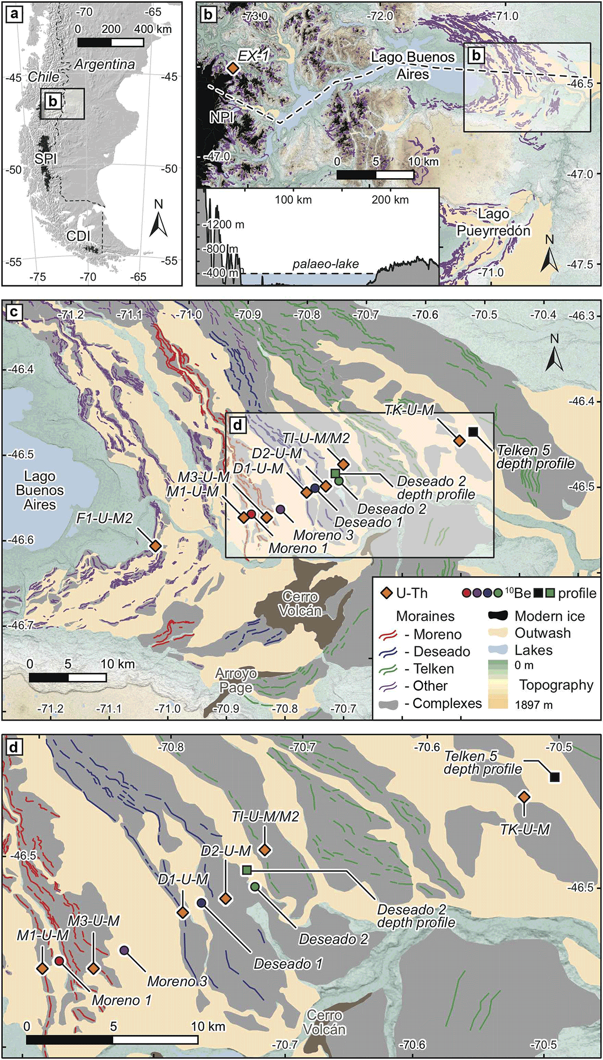
Figure 1Map of the study area adapted from Bendle et al. (2017). (a) Southern South America showing the location of Lago Buenos Aires. The three main contemporary ice masses in Patagonia are also shown: the Northern (NPI) and Southern Patagonian Ice Field (SPI) and the Cordillera Darwin Ice Field (CDI). (b) Inset shows a west–east transect through the study area from the Patagonian Andes to the frontal moraine systems of the proglacial lake (adapted from Kaplan et al., 2009); sample locations as per (a). Panels (c) and (d) show the series of frontal moraines sampled in this study. Silt samples are shown by red circles and cobbles and profiles for cosmogenic analysis are shown in blue; the glacial flour sample at the mouth of Los Exploradores glacier is shown, and the extent of the present day ice field is shown in black. Successive glaciations have formed the large overdeepening in which the proglacial lake has formed.
U and Th samples were taken from silty beds inside the moraines several meters below the surface in order to avoid potential post-depositional modifications, such as weathering or dust inputs (see picture in the Supplement). In addition to moraine samples, a glacial flour sample was taken at the front of the Los Exploradores glacier in Laguna San Rafael National Park to estimate the initial U–Th composition of silts found in the moraines (Fig. 1). This glacier covers part of the total catchment draining into Lago Buenos Aires. Consequently, it is unlikely to be representative of the entire basin but provides an estimate of the initial composition of silts after comminution.
2.2 10Be methodology
2.2.1 Sampling
The cosmogenic nuclide exposure dating methodology followed the sampling recommendations of Hein et al. (2009) and Darvill et al. (2015). We sampled quartzite cobbles for 10Be analysis from the surfaces of outwash grading to the Deseado 1, Deseado 2 and Telken 5 moraines. Similar samples were taken for Moreno 1 and 3 moraines and are presented in Hein et al. (2009). Using outwash cobbles has been shown to overcome issues of post-depositional erosion that affect moraine boulders in this area (Hein et al., 2009), but relies on finding locations where there is a clear geomorphic relationship between the glacial outwash and moraines. At suitable locations, cobbles were targeted based on quartz composition, size (6–15 cm and 300–1 000 g to contain sufficient 10Be) and preservation (sub-rounded shape, little aeolian erosion and partially buried, suggesting they were in situ). Surface lowering or up-freezing of cobbles can result in vertical movement through the outwash unit. In this region, it is more likely that cobbles will underestimate the true age of the unit (Hein et al., 2009, 2017). To circumvent this issue three or four cobbles were analyzed at each sampling location, and the oldest was taken as the best estimate of moraine deposition age.
In addition to cobbles from the outwash surfaces, 10Be depth profiles through exposures within the outwash units were used to estimate surface erosion rates and nuclide inheritance. We sampled through two outwash profiles relating to the Deseado 2 and Telken 5 moraines. Each of the samples making up the depth profiles consisted of 50 to 100 quartz-rich gravel clasts taken from horizontal lines 2–4 cm wide at various depths below the surface. Five depths were sampled per profile between 50 and 240 cm, which is sufficient depth to account for nuclide attenuation from the surface and reliably estimate any cosmogenic 10Be inheritance. The top 50 cm of the profiles were carbonated due to post-depositional processes but the rest of the profiles were of relatively consistent density. See the Supplement for pictures.
2.2.2 Analytical methods
Surface cobbles were analyzed individually as independent estimates of exposure age. The gravels at each depth in the profiles were amalgamated to produce an average nuclide concentration for that depth. Samples were crushed and sieved to obtain the 125–250 µm and the 250–500 µm fractions, which were then purified using a Frantz magnetic separator to isolate non-magnetic fractions. Following dissolution in concentrated HF, the residual sample material was leached with 10 mL H2O to extract Be(OH)2 (Stone, 1998). A combination of anion and cation resins and precipitation was used to purify Be (Norton et al., 2008; von Blanckenburg et al., 2004). The oxidized BeO was mixed with Nb powder, pressed into cathodes and measured on the 0.5 MeV Tandy accelerator at ETH Zürich (Müller et al., 2010). The resulting 10Be∕9Be ratios were normalized to S2007N (Christl et al., 2013; Kubik and Christl, 2010), with a 10Be half-life of 1.387±0.012 Ma (Chmeleff et al., 2010; Korschinek et al., 2010). Measured 10Be∕9Be ratios were 30–500 times higher than the procedure blank (). Blank-corrected 10Be concentrations decrease exponentially with depth from greater than 36×105 at g−1 for near-surface samples to less than 2×10⁵ at g−1 at 2 m of depth.
2.2.3 Deposition age calculations
Exposure ages for the outwash surface cobbles were calculated from 10Be concentrations using version 2.3 of the CRONUS online calculator (Balco et al., 2008). The shielding factor was measured in the field (>0.999999 for every sample), a density of 2.65 g cm−3 was used for every sample and no erosion rate was applied since there were no visible signs of surface erosion. We used the global 10Be production rate of Borchers et al. (2016) (4 ) and the “Lm” scaling scheme (as described in Balco et al., 2008, Lal, 1991, and Stone, 2000, with paleomagnetic corrections from Nishiizumi et al., 1989). However, the scatter between the different scaling schemes is comparable to the external uncertainties. The production rate from Kaplan et al. (2011), calculated from a site very close to LBA, gives 3.6 (Borchers et al., 2016). The difference in calculated exposure ages between these two production rates remains within uncertainties.
We modeled the most probable deposition age, surface erosion rate and nuclide inheritance for each depth profile using the Monte Carlo simulation approach of Hidy et al. (2010). A site production rate of 6.2 was used, taken from an average of the scaling schemes in the CRONUS calculator. Changing this production rate by ±0.3 does not significantly alter the results. This range of site production rates (5.9–6.5 ) corresponds to SLHL production rates of 3.6–4 using the Lm scaling scheme. We used an average profile density of 2.5 g cm−3 (based on field observations) and a shielding factor of 1. The a priori values assigned to the Bayesian Monte Carlo simulation were the following: 0 to 1 cm ka−1 erosion rate with a maximum erosion threshold of 1000 cm and uniform distribution (based on erosion rates in Hein et al., 2009, for the Hatcher profile in nearby Lago Pueyrredón and Darvill et al., 2015); 0 to 105 at g−1 inheritance with uniform distribution (based on concentrations in the lower levels of the profiles); and 200 to 800 ka age range for Deseado 2 and 700 to 1200 ka age range for Telken 5 with uniform distribution. These ages were chosen based on the argon ages of Singer et al. (2004) and the Moreno age refinement of Hein et al. (2017).
2.3 U–Th methodology
2.3.1 Principles and theory
U–Th-series disequilibria have been used for a few decades in order to determine the time constant of weathering. Refer to the Supplement for more references. The comminution age theory introduced by DePaolo et al. (2006) is a promising approach to estimating the age of sediment production. 238U decays into 234Th with a half-life of 4.5 Ga. During this α emission, the daughter isotope recoils over a distance of several tens of nanometers depending on the type of mineral (e.g., 30 nm for a feldspar). 234Th quasi-instantaneously produces 234U, with a longer half-life of 245 kyr, which is long enough to be measurable and usable on geologic timescales. If the 238U decay occurs on the edge of a sediment grain, the daughter isotope is ejected from the grain and a disequilibrium in the decay chain starts as the 234U∕238U ratio of the grain starts to decrease. If the grain is small enough with a large surface area compared to its volume, the disequilibrium can be measured. Steady state is reached after a time characterized by the half-life of 234U. During this transient state, the magnitude of the disequilibrium in a grain equates to the time since it was produced. The steady-state disequilibrium value depends on the fraction of 234U ejected out of the grain due to α recoil. The process can be modeled using the following two equations describing the evolution of 238U and 234U:
λ234 and λ238 are the decay constants of 234U and 238U, respectively. N234 and N238 are the number of nuclides for each isotope, and is the recoil loss fraction of 234U (the proportion of 234U in the grain ejected during α decays). This parameter is critical, since it represents the process that determines the possibility of tracing the comminution age. When the effect of this process starts to be measurable, the clock starts. We discuss in more detail how this parameter can be evaluated in Sect. 2.3.4. The evolution of the U∕Th ratio over time is shown in Fig. 3 (blue curves). The steady-state disequilibrium model is based on the assumption that the sediment grain has not been weathered over time, or at least that the loss of nuclide due to weathering was negligible compared to loss by α recoil. The assumption may be valid for very arid areas, but is otherwise unlikely to hold true. However, the influence of weathering on the comminution age model has not been investigated.
In order to decouple the respective influence of α recoil and weathering, we measured 230Th concentration. The solubility of thorium is much lower than uranium. Therefore the ratio of 230Th∕234U can inform weathering rates. 230Th is produced by 234U decay with a half-life of 75 kyr. It can also be ejected out of the grain due to α recoil. The recoil loss fraction of 230Th, , is related to (Hashimoto et al., 1985; Neymark, 2011).
α230 and α234 are the decay energy of 238U to 234U and of 234U to 230Th, respectively (71.79 and 82.96 keV, respectively). M234 and M230 are the atomic mass of 234U and 230Th. This gives (in practice is probably larger since 234U is on damaged sites, so it increases the probability for 230Th to be ejected from the grain during a decay). The evolution of the number of nuclides 230Th is then given by
Since and λ230>λ234, is always verified. However, weathering would increase the ratio of 230Th∕234U and 230Th∕238U because Th is less soluble than U, and likely decrease the ratio of 234U∕238U because radioactive decay places 234U on a more fragile site compared to 238U so that it could be more easily weathered (DePaolo et al., 2012; Handley et al., 2013a). Consequently, Th isotopes can help to identify and quantify the effects of α recoil and weathering, respectively. New equations can be derived for the evolution of the different nuclide contents following Chabaux et al. (2003, 2008), Dosseto et al. (2008) and Dosseto and Schaller (2016):
where k238, k234 and k230 are the leaching coefficients of 238U, 234U and 230Th, respectively. The solution is shown in Fig. 3.
The steady-state activity ratios can also be derived.
Here, parentheses are used to represent activity ratios corresponding to the isotopic ratio multiplied by the ratio of the respective decay constants of each isotope.
2.3.2 Sample preparation
Silt samples were collected from moraines. Water has likely percolated through these silts since moraine deposition, triggering the precipitation of secondary carbonates, oxides, organic matter and clays. These secondary fractions have different U and Th disequilibria than the primary silicate and it is therefore important to remove them before analysis without altering the primary silicate fraction. We used the protocol established by Lee (2009), with slight modifications to help overcome the low solubility of Th that can make it difficult to remove during successive leaching, and allow Th to adsorb onto mineral surfaces after ejection from the grain. Our protocol is as follows.
-
The samples were sieved at 50 µm in order to collect the ≤50 µm fraction.
-
Approximately 10 g of this fraction was then weighed in a quartz crucible and heated for 4 h at 550 ∘C to burn organic matter. The Lee (2009) optimal protocol uses H2O2 to dissolve organic matter, but other studies have shown that this reagent is not always fully selective (Tessier et al., 1979). The ashing of organic matter yields similar results, but is normally conducted at the end of the procedure (Lee, 2009). By ashing first, we were able to process larger amounts of silt, limiting furnace contamination and aiding the process of dissolving precipitates (mainly oxides formed during heating) in the following steps. Oxides turn the samples a brown to reddish color.
-
Sample grains were dispersed in 0.1 N sodium oxalate and the ≤4 µm fraction was removed using Stokes settling. The ≤4 µm fraction consists of clays and also primary silicates with larger U–Th disequilibria.
-
For each sample, 4 g of sediment was weighed in a 50 mL centrifuge tube and leached twice with 32 mL 1 M magnesium nitrate to remove the exchangeable fraction and any residues of the ashing process.
-
32 mL of acetic acid buffered to pH 5 with 1 M sodium acetate was then added and agitated at room temperature during 5 h to dissolve the carbonates.
-
40 mL of 0.04 M hydroxylamine hydrochloride in 25 % (v∕v) acetic acid was added and heated at 95 ∘C for 6 h twice to dissolve oxides. After this procedure, the samples still had a brown to reddish color from oxides formed in the furnace. These amorphous oxides can be resistant to the hydroxylamine hydrochloride treatment, as shown by Gontier (2014), who recommended using oxalic acid in ammonium oxalate (agitated in the dark at room temperature for 4 h) (Leleyter and Probst, 1999). This procedure preserves silicate from dissolution (Gontier, 2014). Note that for the last three steps, the leaching residues were centrifuged and rinsed twice with MQ water.
At this stage the samples should contain only primary silicates between 4 and 50 µm. To evaluate whether sample preparation fully removed secondary phases (e.g., carbonates, oxides, clays) without affecting primary silicates, we made scanning electron microscopy (SEM) images at the University of Strasbourg, as shown in Sect. 3.2. Our observations showed the method to be effective (see the Supplement for a further discussion on the efficacy of Th removal in this protocol) and the samples were deemed ready for disequilibrium analysis.
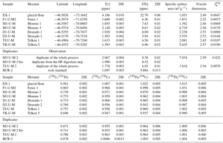
Two duplicates of this pretreatment protocol were measured (see Table 3). They are remarkably consistent within errors for (230Th∕238U) and (230Th∕234U) and only slightly different for (234U∕238U) (only twice the external uncertainty). Since the surface area data are also slightly different, this small difference could be associated with heterogeneities in the powder, fractionation of the grain size during the sampling of the powder or biases in the leaching process.
2.3.3 U–Th disequilibrium analysis
A first aliquot of the samples was dedicated to U–Th analysis. This aliquot was powdered in an agate ball mill to optimize sample homogeneity and acid dissolution. Approximately 100 mg of this powder was spiked with 233U–229Th tracer and digested with concentrated HF–HNO3–HClO4 acids following Pelt et al. (2013). Separation and purification of U and Th followed standard anionic resin chromatography (Dequincey et al., 2002; Granet et al., 2007; Pelt et al., 2008). U and Th isotopic ratios and concentrations were determined by standard sample bracketing (SSB) using an MC-ICPMS Neptune and following an optimized procedure upgraded from previously published protocols (Bosia et al., 2016; Ma et al., 2012; Pelt et al., 2008). The 233U–229Th spike was calibrated against the gravimetric NIST SRM 3164 and 3159 U and Th pure solutions. IRMM-184 and IRMM-035 isotopic standard solutions were spiked and used as bracketing solutions for U and Th SSB analysis, with the 233U∕234U and 229Th∕230Th ratios of these mixtures calibrated by TIMS Triton. We used the consensus value from Sims et al. (2008) for the 232Th∕230Th ratio of the IRMM-035 standard and our own absolute TIMS Triton measurements for the 234U∕238U ratio of the IRMM-184 standard instead of the certified values. The peak tailing of the 232Th over the 230Th was corrected using an exponential law fitted by signals measured in 229.6 and 230.6 masses. The precision and accuracy of the data were estimated from regular analysis of international pure solutions: HU1 for (234U∕238U) at 1.0008±0.0005 (2σ, N=5), IRMM-036 for 232Th∕230Th at 329 064±1313 (2σ, N=5) and rock basalts (BCR-2, AThO and BE-N). Results are consistent with published data and the 238U–234U–230Th secular equilibrium assumed for old (several million years) BCR-2 and BE-N “unweathered” basalts within errors. Based on these pure solutions and homogeneous basalt powders we estimate an uncertainty (2 SD) of 0.2 % for (234U∕238U), 0.5–1 % for (230Th∕232Th) and 1–1.5 % for (238U∕232Th), (230Th∕238U) and (230Th∕234U). A duplicate of the protocol was measured and agrees within the internal measurement uncertainties for (234U∕238U), (230Th∕238U), (230Th∕234U) and a rock standard BCR-2 (see Table 3). Usual blanks in the lab are in the range of 20–50 pg for U and 100–200 pg for Th and are therefore negligible here.
2.3.4 Estimation of the recoil loss factor
The recoil loss parameter (fα) is a critical parameter in comminution age theory as presented in Sect. 2.3.1. Different methods have been proposed to estimate this parameter, as summarized in Maher et al. (2006) and Lee et al. (2010), but discrepancies up to an order of magnitude can be found between the different methods (Handley et al., 2013a, b). Here we used the N2 gas absorption technique, which consists of surface area and fractal dimension measurements. Other methods are more subjective in that they involve visual estimation and assumptions for the aspect ratio and surface roughness coefficient. We measured the specific surface area for all samples and assessed the efficiency of this method to determine fα and the relation between fα and U–Th disequilibria.
A second aliquot of the samples (at least 1 g sample−1) was prepared for these analyses, which were conducted at the Institut de Physique du Globe de Strasbourg on a Carlo Erba Sorptomatic 1990 machine. Details of the procedure are given in the Supplement. Fractal dimensions were also measured for each sample and the recoil loss factor fα was calculated following Bourdon et al. (2009) after Semkow (1991):
where S is the specific surface area, D is the fractal dimension, a is the diameter of the adsorbate molecule (0.35 nm), R is the recoil length (30 nm) and ρs is the density of the solid (2650 kg m−3).
2.3.5 Determination of the recycling time and weathering intensities: Monte Carlo analysis
A Monte Carlo approach was used to determine weathering intensities during both the pre- and post-deposition histories of the different moraine silts, and the duration of this pre-deposition history (called “recycling time” from this point forward).
10Be exposure ages provide information on the deposition age of the moraines. The age extracted from U–Th data provide information on the time since the sediment was produced, so it is equal to the sum of sediment recycling time (time elapsed between comminution and deposition of the moraine) and the deposition age. The problem as formulated in Sect. 2.3.1 has a large number of unknowns compared to the amount of data in each equation, so the problem is underdetermined. However, if geomorphology and climate did not vary too much between each glacial period, we can assume that recycling times and weathering intensities are comparable between the different samples. In fact, the glacial maxima observed since the mid-Pleistocene transition are quite comparable. We can then assume that the processes (especially weathering) occurring during a glacial cycle are comparable in intensity from one cycle to another. Regarding the recycling time, the other main parameter (apart from climate) influencing it is the morphology (mainly valleys and overdeepening). The Great Patagonian Glaciation occurred before 1 Ma (Mercer and Sutter, 1982); these glaciations are most probably responsible for carving the U-shaped valleys and the overdeepening in which the lake is currently. The results of the numerical experiments of Kaplan et al. (2009), regarding the extent of ice related to the elevation of the accumulation area and the depth of the overdeepening, suggest that this overdeepening was most probably already carved before 1 Ma. Recently, Christeleit et al. (2017) argued using thermochronometric data that the relief of Patagonia at the latitudes of our study was probably achieved between 10 and 5 Ma. On that basis, one can assume that the recycling time probably remained constant over the period covered by the samples. Hence all samples are assumed to share the same weathering intensity and the same pre-depositional history duration.
We used the theoretical scheme described in Sect. 2.3.1 to estimate these weathering intensities and recycling times. Known or informed parameters in the Monte Carlo simulations were the activity ratios (234U∕238U) and (230Th∕238U), the initial activity ratio (from the glacial flour sample), the recoil loss factor fα and the deposition ages of the moraines (the post-depositional duration). Unknown parameters were the weathering intensities of 238U, 234U and 230Th for the pre- and post-deposition history. The relative weathering intensity of 234U compared to 238U, and 230Th compared to 238U, were assumed to be the same before and after moraine deposition. Consequently, we needed to determine five unknowns: the respective weathering coefficients , , k234∕k238, k230∕k238 and the recycling time trecycl using Monte Carlo simulations. We chose a large, arbitrary number of values for the unknowns and calculated the activity ratios associated with these sets of values. Then, we calculated a misfit M for the data as the difference between the measured and modeled values weighted by the uncertainty. The lower the misfit, the larger the probability of this set of values (we show the likelihood L for better visibility):
where m is the vector of modeled parameters (the five unknowns above), o is the observed values (the activity ratios (234U∕238U) and (230Th∕238U)) and σ is the diagonal matrix of uncertainties on the data. In theory, an optimal solution can be determined corresponding to the lower misfit (larger likelihood). However, no solutions were found because the number of unknowns was too great. We also know the relative weathering intensities of 238U, 234U and 230Th since Th is less soluble than U and 234U is on more fragile mineralogic sites. Hence, k230 is lower than k238, and k234 is slightly larger than k238. This information was used to further constrain the Monte Carlo simulations. For different couples of k234∕k238 and k230∕k238, we ran a Monte Carlo optimization to find an optimal solution (lower misfit). All optimal solutions for , and the recycling time are shown in Fig. 6, and we use the optimal solutions to characterize the pre-depositional duration of these sediments.
To test whether exchangeable Th might not be efficiently leached by our chemical protocol, we also made a simulation with and (half of the theoretical value described in Sect. 2.3.1). If Th was totally readsorbed onto the mineral surfaces after ejection from the grain (and not subsequently removed during leaching), then it is equivalent to having no ejection (). The case with is an intermediary between total removal of the adsorbed Th and no removal at all, as discussed further in the Supplement.
3.1 Cosmogenic 10Be and deposition ages
The results of 10Be analyses are shown in Fig. 2 and Tables 2 and 1. Refer to the Supplement for more details on the profile age results.
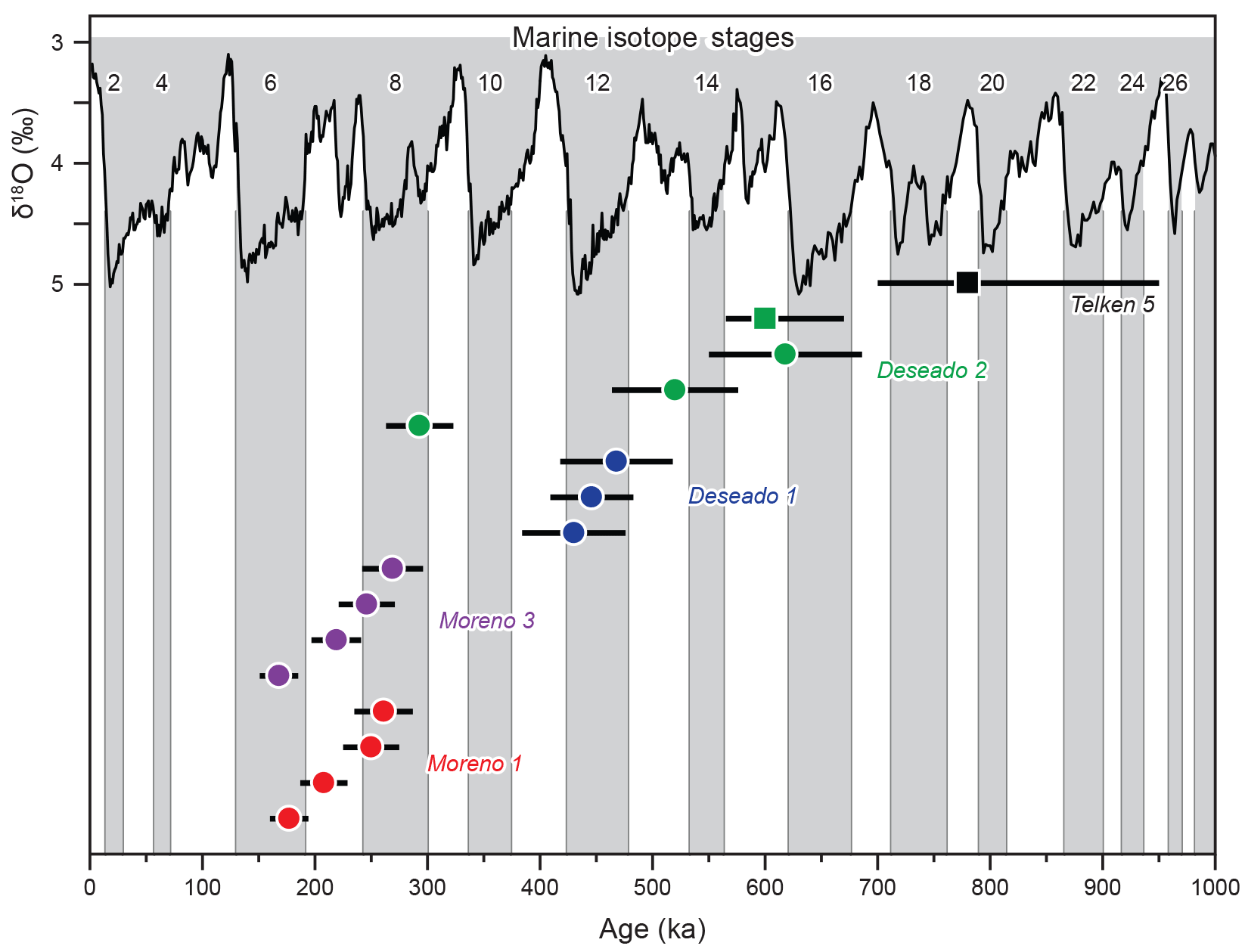
Figure 210Be exposure ages from outwash surface cobbles (circles) and modeled depth profiles (squares) for five of the Lago Buenos Aires moraines. Depth profile uncertainties are 1σ. Symbols and colors are the same as in Fig. 1. The δ18O benthic stack record from Lisiecki and Raymo (2005) is also plotted, and gray shading shows glacial stages.
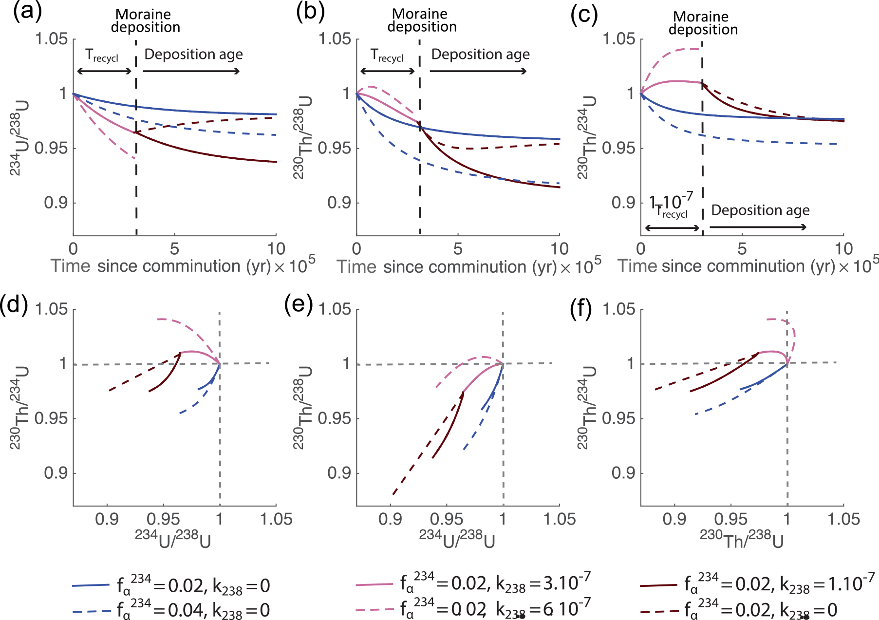
Figure 3Solutions to Eq. 3 that we use as the theoretical framework to analyze our data for different values of fα and k238 (we consider and ). The time evolution of 234U∕238U (a), 230Th∕238U (b) and 230Th∕234U (c) activity ratios. The vertical dashed line represents an event through which the weathering intensity varies: this corresponds in our case to the time of sediment remobilization. Our 10Be exposure ages give the time elapsed since this event (shown by the dashed vertical line), whereas the U–Th data indicate the duration of the first phase since comminution and remobilization (from the x axis origin to the dashed vertical line). (d, e and f) The co-evolution of the ratios in (a), (b) and (c), respectively. Different scenarios are plotted corresponding to different fα values and weathering intensities to illustrate potential patterns in the comminution weathering model (see legend and Sect. 2.3.1). Observing these figures helps in understanding the range of variations in the different activity ratios and the effect of each parameter (α recoil and weathering) on these ratios before and after the remobilization of sediments.
Table 1Cosmogenic 10Be nuclide data for outwash surface cobbles and depth profile samples. Moreno 1 and 3 data are already published in Hein et al. (2017).
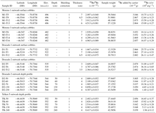
Table 2Modeled exposure ages for outwash surface cobbles and depth profile samples (see main text and the Supplement for details on profile modeling). Moreno 1 and 3 ages have been already published in Hein et al. (2017). Bold values are the oldest samples for each outwash that we consider to be the most representative deposition age of the moraine (see Sect. 3.1 for details).
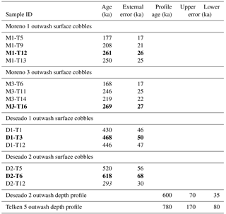
Eight surface cobbles from outwash relating to the Moreno 1 and 3 moraines yielded 10Be exposure ages ranging from 168–269 ka (Hein et al., 2017). To these we add six more surface exposure ages and two depth profile ages from outwash related to the Deseado and Telken moraines. Three cobbles from Deseado 1 produced relatively tightly clustered exposure ages of 430–468 ka. A cobble from the ice-distal Deseado 2 outwash yielded a much younger, stratigraphically inconsistent age of 293 ka (sample D2-T12), similar to the Moreno ages. Two further cobbles from the Deseado 2 outwash yielded ages of 520 and 618 ka, the oldest of which agrees within errors with a modeled depth profile age of 600 ka ( kyr) from the same outwash unit. The agreement between older ages from surface cobbles and the Deseado 2 depth profile is unsurprising given that modeling suggests that surface erosion (<0.2 cm ka−1) and inheritance within the outwash sediments (<2.104 atom g−1) was relatively low (see the Supplement). There are a number of factors that can result in some age scatter within outwash surface cobbles, including surface deflation and up-freezing of clasts (Darvill et al., 2015; Hein et al., 2017). Moreover, Hein et al. (2009, 2017) suggested that the oldest surface exposure ages from outwash in this region will most closely relate to deposition age. The D2-T12 sample is >200 kyr younger than the other Deseado 2 cobbles, and it is likely that this cobble was either deposited at a much later time (perhaps during Moreno-stage glaciation, although the difference in altitude makes this unlikely) or was not in situ. The close agreement between other Deseado 2 ages supports the removal of D2-T12 as an outlier. Finally, a modeled depth profile through outwash relating to the Telken 5 moraine produced an age of 780 ka ( kyr, 1σ confidence interval), with relatively low surface erosion (<0.1 cm ka−1) and inheritance (<6.104 atomg g−1). This age is within the lower range of 760–1016 ka known from radiometric ages (Singer et al., 2004). Sensitivity tests showed that modifications of the a priori values of erosion rates and inheritance lead to insignificant changes in the resulting age.
3.2 Evaluation of the U–Th chemical procedure with SEM images
For three samples taken randomly, we looked at SEM images after 50 µm sieving and preparation (Fig. 4) to assess the effects of our chemical and mechanical treatment. We were particularly interested in whether secondary phases could remain after processing and if the primary silicates could have been altered by this treatment. The minerals observed are mainly quartz, feldspars and micas corresponding to the lithology of the Andes in these latitudes. We list below the main observations.
-
No trace of carbonate, organic matter or oxides were observed in samples that underwent the entire protocol. Prior to treatment, we only note the presence of oxides (Fig. 4b). This does not, however, preclude the presence of carbonate or organic matter since a difference in mass before and after steps 2 and 5 of the protocol was observed. Therefore, the protocol seems efficient at eliminating carbonates, oxides and organic matter.
-
Samples were generally cleaner after preparation. This is because ≤4 µm fractions containing mainly clays were removed by Stokes settling. However, clays are still observed in the samples after preparation (see Fig. 4b and c), mainly agglomerated around primary grains as clay pellets. In one sample, up to one-third of the grains have clay pellets. These clays could have been precipitated directly at the surface of the grains during weathering or agglomerated subsequently. It is difficult to fully eliminate the clays and a potential bias could be introduced if too many clays remain in the sample. This potentially limits the application of comminution ages to samples with a very low amount of clays, since their complete removal is currently not possible.
-
Most micas show surfaces having experienced weathering (Fig. 4d). The shapes observed are typical of weathering both before and after the protocol. This shows that our silt samples have experienced weathering and that it could potentially have affected U–Th disequilibrium.
-
Following the preparation protocol, two feldspar grains in one sample displayed evidence of corrosion (Fig. 4e and f). While this damage could be associated with alteration of the primary silicates during leaching, these are the only two corroded grains visible in the samples we tested. Since the corrosion pits are smaller than 4 µm and all the grains are larger than 4 µm in our samples, ubiquitous damage would be observable on other grains. As such, we assume that primary mineral corrosion during the protocol is minimal.

Figure 4Scanning electron microscopy (SEM) images of selected samples. (a) Overview of a sample after the preparation process described in Sect. 2.3.2. Grains vary in size and shape between 4 and 50 µm and are angular to subangular. White grains are heavy minerals such as zircon or oxides. (b) The same sample before 50 µm sieving. The only notable difference is the presence of clays. (c) Zoomed image of a mineral grain covered in clay pellets that were not removed by the preparation process. (d) Mica grains with cauliflower facies, which is characteristic of weathering. (e, f) Feldspar grains with corroded surfaces. It is unclear whether these corrosion features result from geological processes or the sampling procedure, but they were only observed twice.
3.3 U–Th – fα – age
U–Th results are shown in Fig. 5 and Table 3. (234U∕238U) values from moraines display little variation, ranging from 0.95 to 0.97, while glacial flour has a composition of 1.007 and is close to equilibrium. For the moraine samples, a general decrease in (234U∕238U) is observed with time, though with significant noise. (230Th∕238U) values mostly vary between 0.94 and 0.97 with the youngest moraine sample (F1-U-M2, Fenix moraine) having a composition around 1. Similarly, (230Th∕234U) values mostly range from 0.99 and 1.01, with the youngest moraine around 1.03. Again, an overall decrease in (230Th∕234U) is observed with time. The glacial flour is close to equilibrium compositions with and . Specific surface areas vary from 1.5 to 7 m2 g−1, which is typical for this kind of sample, and the fractal dimensions range from 2.45 to 2.6. The recoil loss factors fα calculated using Eq. 4 are between 0.005 and 0.025, with no observable trend with time.
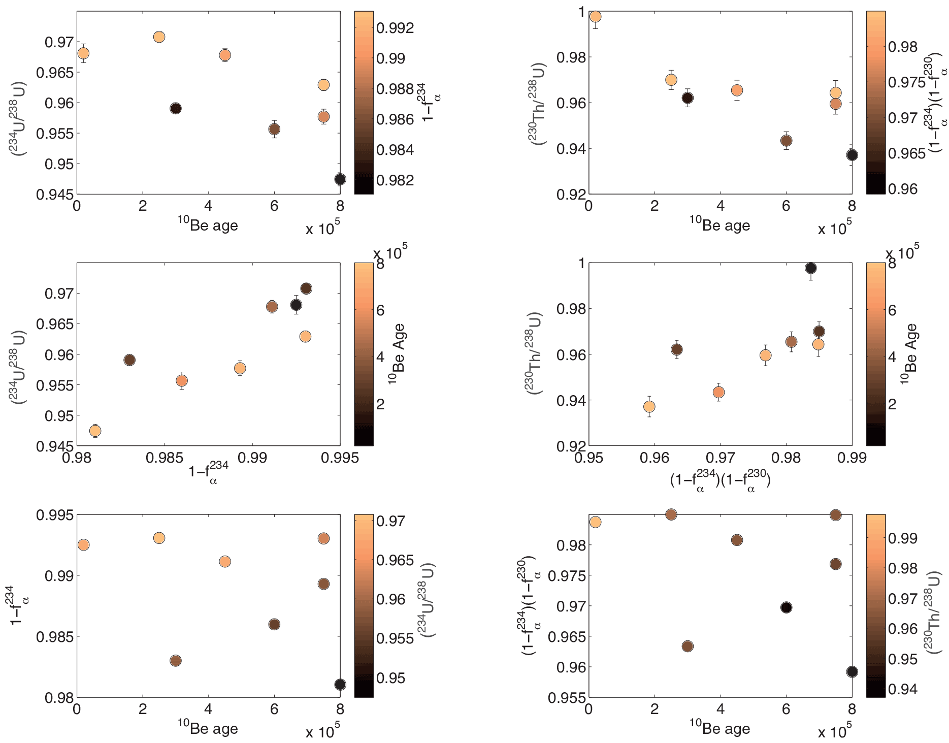
Figure 52-D cross plots of 234U∕238U and 230Th∕238U activity ratios, associated recoil loss factors () and ), and 10Be exposure ages. Symbol colors represent the third parameter in each plot. The sorting observed in the symbol colors helps to explain the noise associated with the other two parameters. In particular, the scatter in the decrease of the activity ratios over time can be largely explained by the variability in the recoil loss factor (top left plot). The plots also let us assume that the variability in the weathering coefficients could be low; otherwise a residual dispersion would be observed. In all cases, error bars are smaller than the size of the dots.
Table 3U–Th concentrations, activity ratios and BET data (specific surface areas, fractal dimensions and calculated recoil loss factors). Duplicates are also shown, two for the whole process (including sieving, leachings, HF digestion and chromatography) and one for HF digestion and chromatography. The samples are sorted by deposition age (F1: Fenix, M1: Moreno 1, M3: Moreno3, D1: Deseado 1, D2: Deseado 2, TI: Telken 1, TK: Telken 5).
Handley et al. (2013a) analyzed only a few samples with the gas adsorption technique to characterize the specific surface area and fα. We analyzed every sample with this technique, highlighting the consistency of the noise in (234U∕238U) and the dispersion in fα derived from specific surface area (Fig. 5). The relationship between (234U∕238U), fα and age is described by a surface in three dimensions. In other words, the noise observed in the (234U∕238U) age diagram around the general decreasing pattern is in large part associated with the dispersion of fα. This suggests that specific surface area data are consistent and reliable or that, if a bias exists in these data, it is systematic. Such a systematic bias would arise from a rather random event due to sample processing, so this latter explanation seems unreasonable. We conclude that the specific surface area determination based on the gas adsorption technique is valid to evaluate the recoil loss factor in the U–Th comminution age theory.
We observe that (230Th∕234U) is larger than (234U∕238U) and (230Th∕238U) has comparable compositions to (234U∕238U). As mentioned in Sect. 2.3.1, this observation is incompatible with a simple comminution age model (only α recoil). An enrichment of 230Th compared to 234U could be the imprint of weathering on silts found in the moraines. Similarly, the incompatibilities of (234U∕238U) and fα in the framework of the simple comminution age model suggest that weathering must be considered. In the comminution age theory as described by DePaolo et al. (2006), 1−fα must always be lower than (234U∕238U), and for a sample old enough to have reached steady state, . This is not what we observe, similarly to Handley et al. (2013a). However, as described in Sect. 2.3.1 such an observation can be explained if weathering is considered and k234≥k238.
Given the large disequilibrium of the youngest samples in (234U∕238U) and in (230Th∕234U) (Table 3 and Fig. 5) and the fact that the glacial flour (the most probable initial composition for the moraine silts) is close to equilibrium, we cannot ignore the pre-depositional history (i.e., before deposition in the moraines). Based on a starting value close to equilibrium, the disequilibrium values measured here cannot be reached in only 20 or even 200 kyr. Since our estimations of the fα seem consistent and reliable, this requires consideration of a pre-depositional history involving weathering with a different intensity than during the post-deposition history.
3.4 Pre-deposition history and Monte Carlo analysis
We attempt to constrain the pre-depositional history using a Monte Carlo analysis. The results show an inverse relationship, with the greatest probability for between 2 and 3 and a recycling time between 100 and 200 kyr. The optimal values of k234∕k238 and k230∕k238 associated with this solution describe an anticorrelation with and (Fig. 6). These parameters are, however, poorly constrained by the inversion process.
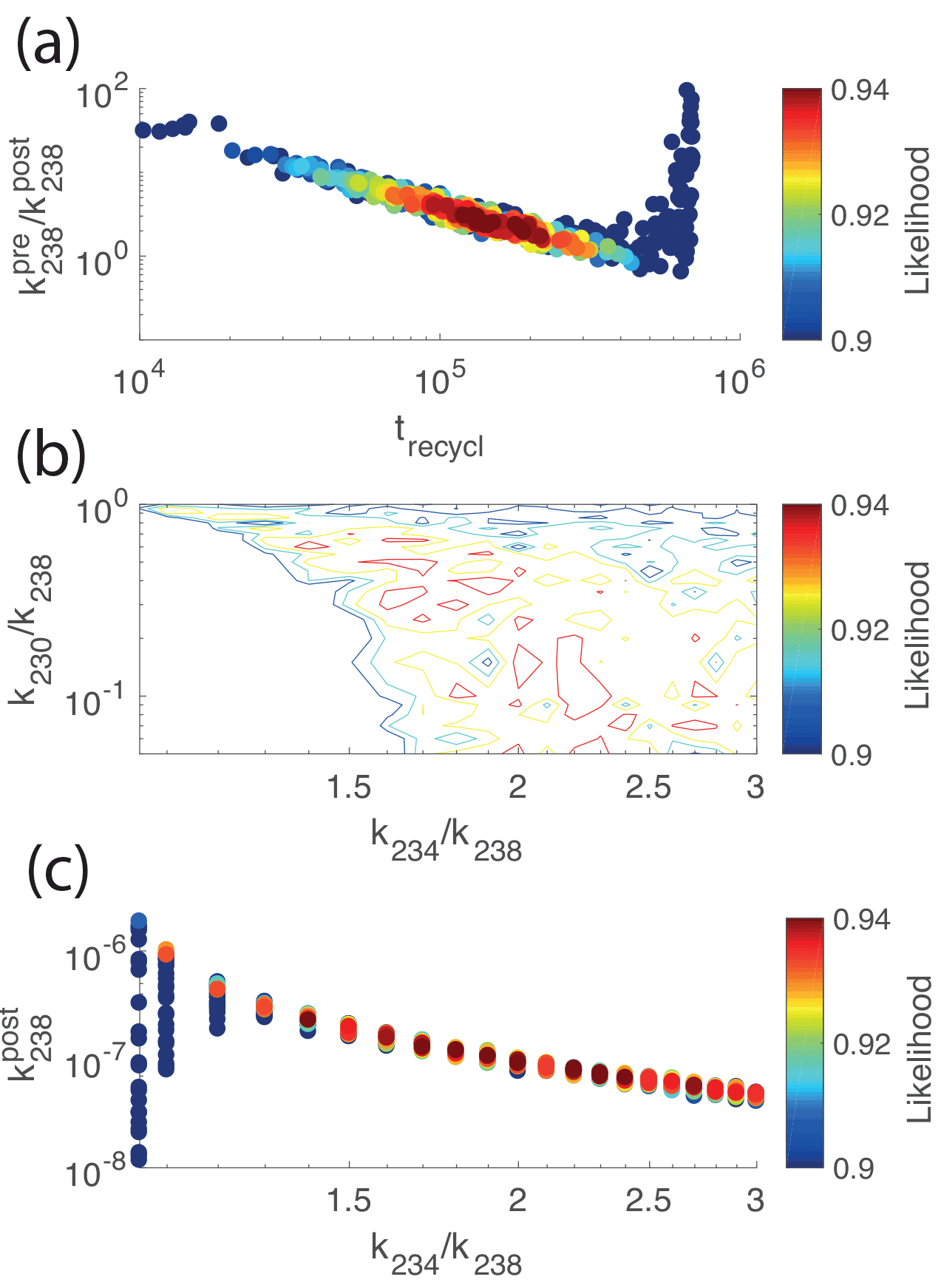
Figure 6Results of Monte Carlo simulations for the U–Th data. The same Monte Carlo simulations were conducted for different fixed values of k234∕k238 and k230∕k238 (see Sect. 2.3.5). For each simulation we estimated the optimal solution for , and recycling time (pre-deposition duration, after comminution), i.e., the solution with the lowest misfit between measured and calculated activity ratio data. We used this misfit to calculate a likelihood between 0 and 1 (see Eq. 5), as shown by the color map (red is lower misfit, blue is higher misfit; stretched to fit our results). The larger the likelihood, the closer to the data the solution is, so the more likely the set of parameter values. (a) The ratio as a function of the recycling time. Each dot is one Monte Carlo solution. The optimal solution (red dots) is for 3 times stronger weathering before deposition and a recycling time of 100 kyr. (b) Relative weathering intensities of 234U, 238U and 230Th. The relative weathering intensities are poorly constrained, but a relationship can be extracted between their ratios: the larger k234∕k238, the smaller k230∕k238 must be. (c) A relation between and k234∕k238 can be extracted, even if both parameters are poorly constrained. The estimation of sediment transfer times using U–Th disequilibria series could be improved with better constraints on the relative mobility of 234U and 238U.
Despite the numerous parameters to be constrained, the model converges for key results as shown above. We show in particular that, in the framework of the modified comminution age theory incorporating weathering, as described in Sect. 2.3.1, the silts from the LBA moraines were likely eroded 100 to 200 kyr before being deposited in the moraines and that on average they experienced around 2–3 times more intense weathering during this interval than after deposition (Fig. 6). The best fit corresponding to a recycling time of 180 kyr, a ratio , and , is shown in the Supplement Fig. S5.
4.1 Glacial chronology and perspectives on the control of ice extent in the Patagonian Andes
The new 10Be exposure ages in this study help clarify the timing of the deposition of several LBA moraines. The oldest outwash cobbles are taken as closest to the age of deposition because depth profiles show that average nuclide inheritance is relatively low and outwash surfaces show evidence of deflation (Hein et al., 2011, 2017). It is possible that even the oldest cobbles underestimate the age of deposition if they have also been exhumed, and we apply no erosion correction to our exposure ages. As discussed in Hein et al. (2017), outwash surface cobbles imply that the Moreno moraines were deposited at ca. 260–270 ka during marine isotope stage 8.
Unlike the Moreno system, surface cobbles from the Deseado moraines appear to date from two different glacial cycles. Exposure ages from Deseado 1 outwash yield relatively tightly clustered ages of 430–470 ka, suggesting that the limit was deposited during MIS 12. The older of two published moraine boulder exposure ages from the Deseado 1 moraine (Kaplan et al., 2005) is consistent with the cobble ages in this study. In contrast, surface cobbles from Deseado 2 outwash yield ages of 520 and 618 ka (excluding the anomalously young D2-T12 age of 293 ka). The dating would be less conclusive without the accompanying depth profile age of 600 ka kyr. Slight changes in scaling factors (see Sect. 2.2.3) do not affect this finding. Taken together, the oldest surface cobble and depth profile suggest that the Deseado 2 limit was deposited at ca. 600–620 ka. Within errors, the limit may relate to MIS 16. The scatter in ages is interesting given that luminescence dating yielded an even younger age of 123±18 ka for the Deseado 2 limit (Smedley et al., 2016). This scatter may imply greater sediment reworking or a more complex relationship between moraines and outwash in this sequence. The Telken 5 depth profile gave an age of 780 ka kyr that is stratigraphically consistent within our chronological dataset, but less helpful in determining when the limit was deposited. The error range spans MIS 18–24 (and radiometric datings gave a lower age of 760 ka for the Telken series), with larger probability around MIS 20, so it is possible that the moraine was deposited during MIS 20. Since the entire Telken moraine system must be older than 760 ka (Singer et al., 2004), this implies that Telken 1 to 4 are also that age and that the Telken moraines represent different glacial advances during the same glacial cycle.
In summary, there is a clear pattern in the timing of moraine deposition in which alternate glacial cycles are represented in our chronology: Telken 5 during MIS 20; Deseado 2 during MIS 16; Deseado 1 during MIS 12; and the Moreno moraines during MIS 8. Previous work has shown that the innermost Fenix moraines relate to the Last Glacial Maximum during MIS 2 (Douglass et al., 2006; Kaplan et al., 2004; Smedley et al., 2016). We strongly caution that scatter in surface cobble ages and error ranges in depth profiles may complicate this pattern, particularly for the older limits. Moreover, we did not analyze the enigmatic Deseado 3 moraine and so cannot say whether this relates to the counterparts dated here or intervening glacial stages. However, the dating of the Moreno and Deseado 1 and 2 moraines does imply that the intervening glacial cycle is absent from the record.
The pattern in the timing of moraine deposition around Lago Buenos Aires implies that there are a few glacial cycles that are either not recorded in this area or have been erased or removed. Either the ice lobe did not advance during alternate glacial cycles, or it advanced to similar or less extensive positions so that moraines and outwash were then removed by the following advance. A similar pattern was observed by Hein et al. (2009, 2011) for the Lago Pueyrredón ice lobe 100 km to the south, so there could be a regional driver of alternate glacial advances. One possibility is that erosion over successive glacial cycles caused entrenchment of ice lobes within large basins on the eastern side of the Patagonian Ice Sheet (Kaplan et al., 2009). This erosion model has been linked to the pattern of nested limits seen across the former ice sheet (Anderson et al., 2012; Kaplan et al., 2009) but may be more complex if only alternate cycles are represented in the moraine record. Alternatively, a purely climatic forcing could have caused alternate strong advances, although there is no simple relationship between available climate records and alternate glacial advances at Lago Buenos Aires. A complex erosion–climate feedback mechanism may determine when or how far glacial advances occurred in this region, but more detailed glacial models are required to further test such a model.
The chronology presented here suggests that moraine reworking has probably occurred in the area and/or that glacial erosion in the Andes may feed back into the glacial lobe advance to produce this observed pattern of absent intervening glacial cycles. Regardless, this chronology allows us to broadly constrain deposition ages of moraines targeted for U–Th analysis, which may in turn inform sediment recycling times between preserved moraines.
4.2 Implications for sediment recycling, chemical weathering, climate and their interactions in proglacial systems
Following the conclusions of Handley et al. (2013a), the residence time of 100–200 kyr could be an artifact due to an addition of old dust. In our area, when a new moraine is being formed, the older sediments are on the east, whereas the dominant winds come from the west. It is therefore unlikely that these winds could add older material to that being deposited.
The long time estimated using the whole set of data and the Monte Carlo simulations, along with the absence of inheritance in the 10Be data, suggest that the sediment was not exposed at the surface in the proglacial system before being deposited in its moraine. This implies that the sediment must have been buried, either in the proglacial lake or within a sedimentary pile (moraine, till, channel, etc., at least a few meters below the surface) before final deposition.
The dated sediment was most probably eroded during glacial periods, as erosion rates are likely much larger than during an interglacial. Likewise, deposition in an end moraine occurs during a glacial period. This means that the sediment deposited in the moraine may spend on average as long as 100–200 kyr in the proglacial system (till, lake sediments, etc.) before being deposited in the moraines. Hence the sediment eroded during a glacial period is on average deposited in the frontal moraine during the next glacial cycle. Using postglacial sediment budget and reservoir theory, Hoffmann and Hillebrand (2016) modeled the residence time of sediments in a periglacial system in the Canadian Rocky Mountains and also found a time of 100 kyr. This average residence time implies that a fraction of the sediment deposited in a moraine may have been produced during the same glacial cycle with another fraction being much older.
This time appears to be long. However, our measurements of cosmogenic exposure ages using 10Be nuclide concentrations in outwash cobbles and profiles suggest that the preserved moraines represent every other glacial cycle, indicating an advance over the proglacial sediment of one or two previous advances. Moreover, it has been shown that proglacial lakes occupying overdeepenings are filled following deglaciation (Eyles et al., 1991; Houbolt and Jonker, 1968). The lakes are filled with sediments during interglacial periods and emptied during the subsequent glacial periods. These processes imply sediment erosion and deposition over a full glacial–interglacial cycle, which is consistent with both 10Be and U–Th disequilibrium data.
We also obtain a weathering rate that is 2–3 times higher during the 100–200 kyr of the pre-depositional phase than after deposition. Based on the argument above, these sediments are exposed to water in the proglacial system before deposition in the moraine. Authors such as Anderson (2005) have shown that proglacial environments favor weathering. Since weathering rate is a time-dependent parameter (White and Brantley, 2003), the calculated recycling time of 100–200 kyr likely has a non-negligible impact on weathering fluxes.
Understanding how sediments are evacuated and transported to the oceans and when they experience weathering would help to quantify the relationships between erosion and climate. In particular, if 100 to 200 kyr are needed to escape the periglacial area, important lags could be observed between an erosional forcing and the weathering and climate response. This suggests that measured weathering variations could have occurred over the last glacial–interglacial cycles or could have been smoothed and/or damped because of a lag in the sediment transport. Estimating these lag times would help in understanding the relationships between erosion, climate and marine biogeochemical cycles. Erosion rates can be determined using thermochronology or cosmogenic isotopes. Sedimentation rates in the ocean can also be estimated using marine core dating methods. The link between erosion and sedimentation is poorly known (Sadler, 1981), especially because the transport times are poorly constrained. The transport time of 100 to 200 kyr presented here suggests that the pathway between initial erosion and deposition is potentially complex. An effort to constrain these transport times appears to be potentially fruitful to reveal the actual link between erosion and sedimentation rates and climate.
4.3 Perspectives on comminution age method and its applications to characterize sediment transfer
Our data let us estimate only a mean recycling time for moraine sediment (the fine silty fraction). Here we have discussed it in terms of the recycling of the previous glacial cycle moraine, but it could also be interpreted as a mixing of much older, deeper, reworked sediment with new freshly eroded sediment. In other words, we do not quantify the amount of sediment escaping the proglacial system or the amount of sediment rapidly deposited in the moraine after erosion. It would be beneficial to think about age distributions and not only mean ages. However, this necessitates being able to measure U–Th disequilibrium on single grains, which remains an analytical challenge (Bosia et al., 2018).
Quantifying or reducing the effects of weathering remains a major challenge. Pure primary minerals with no clays would minimize these secondary processes. To this end, working on pure zircon grains could be an option. This would require improved mineral separation methods for fractions smaller than 50 µm. One would also have to assume that comminution effectively occurred on such a heavy mineral and that there is no initial disequilibrium (a problem being that zircons are much more enriched in U than the surrounding minerals).
Our study is a first attempt to quantify long-term sediment transfer times in a proglacial area. We take advantage of the particularly well-preserved series of nested moraines of the Lago Buenos Aires in Patagonia. Our approach involves 10Be exposure dating of these moraines combined with U–Th disequilibrium measurement on the fine fraction of moraine sediment, within a “modified” comminution theoretical framework, to characterize the pre-deposition and post-deposition histories of the sediments.
We show that weathering cannot be neglected when determining the comminution age. Measuring Th isotopes helps constrain the weathering process. Even with this complication, it is possible to calculate comminution ages if the studied samples have well-constrained deposition ages and have experienced the same pre-depositional history. In this case, both the weathering intensities and the pre-depositional history duration are the same for all the samples. We also show that specific surface area measurements based on the gas adsorption technique for estimation of the recoil loss factor is a reliable method and should be applied to all samples. One caveat is that clay minerals may not be removed from the samples, especially clay pellets agglomerated at some mineral surfaces, which could be a strong limitation of the use of this method to calculate transport times.
Our new chronology shows that some glacial cycles are either not preserved or not recorded in the LBA area; i.e., the associated moraines may have been removed by following glacial advances or may have been deposited farther upstream. Hein et al. (2011) found a similar pattern in the Lago Pueyrredón area, suggesting that the mechanisms driving glacial advance may have a regional extent. Future work may reveal whether erosion feedbacks in the Andes could be responsible for this pattern.
The absence of moraine records for a few glacial cycles in the LBA area can be explained by our U–Th data showing that there has been reworking and/or recycling of the sediments. Using a Monte Carlo approach we estimate that the silts from the Lago Buenos Aires frontal moraine system have a 100 kyr residence time in the proglacial system (transported in the lake sediments, remobilized from the previous moraines or stored in intermediate reservoirs) and experienced 3 times more intense weathering before deposition than in the moraine. Our data represent a step forward in the effort to constrain the pathways and timescales over which sediments are transported from source (erosion in mountain belts) to sink (ocean sediments). Although considered a daunting challenge by Sadler and Jerolmack (2015) and requiring additional development, this approach can contribute to our understanding of basin-scale sediment budgets and how erosion, weathering and sedimentation evolve through time.
All data discussed in this paper and relevant references are available in the indicated tables.
The supplement related to this article is available online at: https://doi.org/10.5194/esurf-6-121-2018-supplement.
The authors declare that they have no conflict of interest.
We thank the administration of the Laguna San Rafael National Park
for granting us the authorization to sample in the Los
Exploradores glacier area, especially Cristobal Fabres for his kind
support and accompaniment during the sampling.
Edited by: Jane Willenbring
Reviewed by: two anonymous referees
Ackerer, J., Chabaux, F., Van der Woerd, J., Viville, D., Pelt, E., Kali, E., Lerouge, C., Ackerer, P., di Chiara Roupert, R., and Négrel, P.: Regolith evolution on the millennial timescale from combined U–Th–Ra isotopes and in situ cosmogenic 10Be analysis in a weathering profile (Strengbach catchment, France), Earth Planet. Sc. Lett., 453, 33–43, 2016. a
Andersen, M. B., Vance, D., Keech, A., Rickli, J., and Hudson, G.: Estimating U fluxes in a high-latitude, boreal post-glacial setting using U-series isotopes in soils and rivers, Chem. Geol., 354, 22–32, 2013. a
Anderson, R., Dühnforth, M., Colgan, W., and Anderson, L.: Far-flung moraines: Exploring the feedback of glacial erosion on the evolution of glacier length, Geomorphology, 179, 269–285, 2012. a
Anderson, S.: Glaciers show direct linkage between erosion rate and chemical weathering fluxes, Geomorphology, 67, 147–157, 2005. a, b
Anderson, S., Drever, J., and Humphrey, N.: Chemical weathering in glacial environments, Geology, 25, 399–402, 1997. a
Balco, G., Stone, J., Lifton, N., and Dunai, T.: A complete and easily accessible means of calculating surface exposure ages or erosion rates from 10Be and 26Al measurements, Quat. Geochronol., 3, 174–195, 2008. a, b, c
Bendle, J., Thorndycraft, V., and Palmer, A.: The glacial geomorphology of the lago Buenos Aires and lago Pueyrredón ice lobes of central Patagonia, J. Maps, 13, 654–673, 2017. a
Borchers, B., Marrero, S., Balco, G., Caffee, M., Goehring, B., Lifton, N., Nishiizumi, K., Phillips, F., Schaefer, J., and Stone, J.: Geological calibration of spallation production rates in the cronus-earth project, Quat. Geochronol., 31, 188–198, 2016. a, b
Bosia, C., Chabaux, F., Pelt, E., France-Lanord, C., Morin, G., Lavé, J., and Stille, P.: U–Th-Rra variations in himalayan river sediments (Gandak river, India): Weathering fractionation and/or grain-size sorting?, Geochim. Cosmochim. Ac., 193, 176–196, 2016. a
Bosia, C., Chabaux, F., Pelt, E., Cogez, A., Stille, P., Deloule, E., and France-Lanord, C.: U-series disequilibria in minerals from gandak river sediments (Himalaya), Chem. Geol., 477, 22–34, 2018. a
Bourdon, B., Bureau, S., Andersen, M., Pili, E., and Hubert, A.: Weathering rates from top to bottom in a carbonate environment, Chem. Geol., 258, 275–287, 2009. a
Chabaux, F., Riotte, J., and Dequincey, O.: U-Th-Ra fractionation during weathering and river transport, Rev. Mineral. Geochem., 52, 533–576, 2003.
Chabaux, F., Bourdon, B., and Riotte, J.: U-series geochemistry in weathering profiles, river waters and lakes, Radioactiv. Environm., 13, 49–104, 2008. a
Chabaux, F., Blaes, E., Granet, M., di Chiara Roupert, R., and Stille, P.: Determination of transfer time for sediments in alluvial plains using 238U-234U-230Th disequilibria: The case of the Ganges river system, CR Geosci., 344, 688–703, 2012. a
Chabaux, F., Blaes, E., Stille, P., di Chiara Roupert, R., Pelt, E., Dosseto, A., Ma, L., Buss, H., and Brantley, S.: Regolith formation rate from U-series nuclides: implications from the study of a spheroidal weathering profile in the Rio Icacos watershed (Puerto Rico), Geochim. Cosmochim. Ac., 100, 73–95, 2013. a
Chmeleff, J., von Blanckenburg, F., Kossert, K., and Jakob, D.: Determination of the 10Be half-life by multicollector icp-ms and liquid scintillation counting, Nucl. Instrum. Meth. B, 268, 192–199, 2010. a
Christeleit, E., Brandon, M., and Shuster, D.: Miocene development of alpine glacial relief in the patagonian Andes, as revealed by low-temperature thermochronometry, Earth Planet. Sc. Lett., 460, 152–163, 2017. a
Christl, M., Vockenhuber, C., Kubik, P., Wacker, L., Lachner, J., Alfimov, V., and Synal, H.-A.: The ETH Zurich AMS facilities: Performance parameters and reference materials, Nucl. Instrum. Meth. B, 294, 29–38, 2013. a
Cogez, A., Meynadier, L., Allègre, C., Limmois, D., Herman, F., and Gaillardet, J.: Constraints on the role of tectonic and climate on erosion revealed by two time series analysis of marine cores around New Zealand, Earth Planet. Sc. Lett., 410, 174–185, 2015. a
Darvill, C. M., Bentley, M. J., Stokes, C. R., Hein, A. S., and Rodés, Á.: Extensive mis 3 glaciation in southernmost Patagonia revealed by cosmogenic nuclide dating of outwash sediments, Earth Planet. Sc. Lett., 429, 157–169, 2015. a, b, c, d
DePaolo, D., Maher, K., Christensen, J., and McManus, J.: Sediment transport time measured with U-series isotopes: results from ODP north Atlantic drift site 984, Earth Planet. Sc. Lett., 248, 394–410, 2006. a, b, c
DePaolo, D. J., Lee, V. E., Christensen, J. N., and Maher, K.: Uranium comminution ages: Sediment transport and deposition time scales, CR Geosci., 344, 678–687, 2012. a, b
Dequincey, O., Chabaux, F., Clauer, N., Sigmarsson, O., Liewig, N., and Leprun, J.-C.: Chemical mobilizations in laterites: evidence from trace elements and 238U–234U–230Th disequilibria, Geochim. Cosmochim. Ac., 66, 1197–1210, 2002. a
Dosseto, A. and Schaller, M.: The erosion response to quaternary climate change quantified using uranium isotopes and in situ-produced cosmogenic nuclides, Earth-Sci. Rev., 155, 60–81, 2016. a
Dosseto, A., Bourdon, B., and Turner, S. P.: Uranium-series isotopes in river materials: insights into the timescales of erosion and sediment transport, Earth Planet. Sc. Lett., 265, 1–17, 2008.
Dosseto, A., Hesse, P., Maher, K., Fryirs, K., and Turner, S.: Climatic and vegetation control on sediment dynamics during the last glacial cycle, Geology, 38, 395–398, 2010. a, b
Dosseto, A., Buss, H., and Suresh, P.: Rapid regolith formation over volcanic bedrock and implications for landscape evolution, Earth Planet. Sc. Lett., 337, 47–55, 2012. a
Dosseto, A., Buss, H., and Chabaux, F.: Age and weathering rate of sediments in small catchments: The role of hillslope erosion, Geochim. Cosmochim. Ac., 132, 238–258, 2014. a
Douglass, D., Singer, B., Kaplan, M., Mickelson, D., and Caffee, M.: Cosmogenic nuclide surface exposure dating of boulders on last-glacial and late-glacial moraines, lago Buenos Aires, Argentina: interpretive strategies and paleoclimate implications, Quat. Geochronol., 1, 43–58, 2006. a, b
Ebelmen, J.: Sur les produits de la décomposition des espèces minérales de la famille des silicates, Ann. Mines, 7, 3–66, 1845. a
Eyles, N., Mullins, H., and Hine, A.: The seismic stratigraphy of Okanagan lake, British Columbia; a record of rapid deglaciation in a deep “fiord-lake” basin, Sediment. Geol., 73, 13–41, 1991. a
Foster, G. and Vance, D.: Negligible glacial–interglacial variation in continental chemical weathering rates, Nature, 444, 918–921, 2006. a
Gontier, A.: Quantification de l'altération dans les sols par les déséquilibres radioactifs: approche sur sol total et phases minérales séparées, PhD thesis, University of Strasbourg, France, 2014. a, b
Granet, M., Chabaux, F., Stille, P., France-Lanord, C., and Pelt, E.: Time-scales of sedimentary transfer and weathering processes from U-series nuclides: clues from the himalayan rivers, Earth Planet. Sc. Lett., 261, 389–406, 2007. a
Granet, M., Chabaux, F., Stille, P., Dosseto, A., France-Lanord, C., and Blaes, E.: U-series disequilibria in suspended river sediments and implication for sediment transfer time in alluvial plains: the case of the himalayan rivers, Geochim. Cosmochim. Ac., 74, 2851–2865, 2010. a
Hallet, B., Hunter, L., and Bogen, J.: Rates of erosion and sediment evacuation by glaciers: a review of field data and their implications, Global Planet. Change, 12, 213–235, 1996. a
Handley, H., Turner, S., Afonso, J., Dosseto, A., and Cohen, T.: Sediment residence times constrained by uranium-series isotopes: a critical appraisal of the comminution approach, Geochim. Cosmochim. Ac., 103, 245–262, 2013a. a, b, c, d, e, f
Handley, H., Turner, S., Dosseto, A., Haberlah, D., and Afonso, J.: Considerations for U-series dating of sediments: Insights from the flinders ranges, South Australia, Chem. Geol., 340, 40–48, 2013b. a, b
Hashimoto, T., Aoyagi, Y., Kudo, H., and Sotobayashi, T.: Range calculation of alpha-recoil atoms in some minerals using lss-theory, J. Radioanal. Nucl. Ch., 90, 415–438, 1985. a
Hein, A., Hulton, N., Dunai, T., Schnabel, C., Kaplan, M., Naylor, M., and Xu, S.: Middle Pleistocene glaciation in Patagonia dated by cosmogenic-nuclide measurements on outwash gravels, Earth Planet. Sc. Lett., 286, 184–197, 2009. a, b, c, d, e, f, g
Hein, A., Dunai, T., Hulton, N., and Xu, S.: Exposure dating outwash gravels to determine the age of the greatest patagonian glaciations, Geology, 39, 103–106, 2011. a, b, c
Hein, A., Cogez, A., Darvill, C., Mendelova, M. R., Kaplan, M., Herman, F., Dunai, T., Norton, K., Xu, S., Christl, M., and Rodes, A.: Regional Mid-Pleistocene glaciation in central patagonia, Quaternary Sci. Rev., 164, 77–94, 2017. a, b, c, d, e, f, g, h, i, j
Hidy, A., Gosse, J., Pederson, J., Mattern, J., and Finkel, R.: A geologically constrained monte carlo approach to modeling exposure ages from profiles of cosmogenic nuclides: An example from Lees Ferry, Arizona, Geochem. Geophy. Geosy., 11, https://doi.org/10.1029/2010GC003084, 2010. a
Hoffmann, T. and Hillebrand, G.: Sediment residence time and connectivity in non-equilibrium and transient geomorphic systems, EGU General Assembly Conference Abstracts, 18, 609–627, 2016. a
Houbolt, J. and Jonker, J.: Recent sediments in the eastern part of the lake of Geneva (Lac Leman), Geol. Mijnbouw, 47, 131–148, 1968. a
Kaplan, M., Ackert, R., Singer, B., Douglass, D., and Kurz, M.: Cosmogenic nuclide chronology of millennial-scale glacial advances during O-isotope stage 2 in Patagonia, Geol. Soc. Am. Bull., 116, 308–321, 2004. a, b
Kaplan, M., Douglass, D., Singer, B., Ackert, R., and Caffee, M.: Cosmogenic nuclide chronology of pre-last glacial maximum moraines at Lago Buenos Aires, 46 S, Argentina, Quaternary Res., 63, 301–315, 2005. a, b, c
Kaplan, M., Hein, A., Hubbard, A., and Lax, S.: Can glacial erosion limit the extent of glaciation?, Geomorphology, 103, 172–179, 2009. a, b, c, d, e
Kaplan, M., Strelin, J., Schaefer, J., Denton, G., Finkel, R., Schwartz, R., Putnam, A., Vandergoes, M., Goehring, B., and Travis, S.: In-situ cosmogenic 10Be production rate at Lago Argentino, Patagonia: implications for late-glacial climate chronology, Earth Planet. Sc. Lett., 309, 21–32, 2011. a
Keech, A., West, A., Pett-Ridge, J., and Henderson, G.: Evaluating U-series tools for weathering rate and duration on a soil sequence of known ages, Earth Planet. Sc. Lett., 374, 24–35, 2013. a
Koppes, M. and Montgomery, D.: The relative efficacy of fluvial and glacial erosion over modern to orogenic timescales, Nat. Geosci., 2, 644–647, 2009. a
Korschinek, G., Bergmaier, A., Faestermann, T., Gerstmann, U., Knie, K., Rugel, G., Wallner, A., Dillmann, I., Dollinger, G., Von Gostomski, C., Kossert, K., Maiti, M., Poutivtsev, M., and Remmert, A.: A new value for the half-life of 10Be by heavy-ion elastic recoil detection and liquid scintillation counting, Nucl. Instrum. Meth. B, 268, 187–191, 2010. a
Kubik, P. W. and Christl, M.: 10Be and 26Al measurements at the Zurich 6mv tandem AMS facility, Nucl. Instrum. Meth. B, 268, 880–883, 2010. a
Lal, D.: Cosmic ray labeling of erosion surfaces: in-situ nuclide production rates and erosion models, Earth Planet. Sc. Lett., 104, 424–439, 1991. a, b
Lee, V., DePaolo, D., and Christensen, J.: Uranium-series comminution ages of continental sediments: Case study of a Pleistocene alluvial fan, Earth Planet. Sc. Lett., 296, 244–254, 2010. a, b
Lee, V. E.: Radiogenic isotope geochemistry and the evolution of the Earth's surface and interior, PhD thesis, University of California, Berkeley, USA, 2009. a, b, c
Leleyter, L. and Probst, J.: A new sequential extraction procedure for the speciation of particulate trace elements in river sediments, Int. J. Environ. An. Ch., 73, 109–128, 1999. a
Lisiecki, L. and Raymo, M.: A Pliocene-Pleistocene stack of 57 globally distributed benthic δ18O records, Paleoceanography, 20, 2005. a
Lupker, M., France-Lanord, C., Galy, V., Lavé, J., and Kudrass, H.: Increasing chemical weathering in the himalayan system since the last glacial maximum, Earth Planet. Sc. Lett., 365, 243–252, 2013. a
Ma, L., Chabaux, F., Pelt, E., Granet, M., Sak, P. B., Gaillardet, J., Lebedeva, M., and Brantley, S. L.: The effect of curvature on weathering rind formation: Evidence from uranium-series isotopes in basaltic andesite weathering clasts in Guadeloupe, Geochim. Cosmochim. Ac., 80, 92–107, 2012. a
Ma, L., Chabaux, F., West, N., Kirby, E., Jin, L., and Brantley, S.: Regolith production and transport in the Susquehanna Shale Hills critical zone observatory. Part 1: Insights from U-series isotopes, J. Geophys. Res.-Earth, 118, 722–740, 2013. a
Maher, K., DePaolo, D., and Christensen, J.: U–Sr isotopic speedometer: fluid flow and chemical weathering rates in aquifers, Geochim. Cosmochim. Ac., 70, 4417–4435, 2006. a, b
Mercer, J. and Sutter, J. F.: Late Miocene – earliest Pliocene glaciation in southern Argentina: implications for global ice-sheet history, Palaeogeogr. Palaeocl., 38, 185–206, 1982. a, b
Müller, A., Christl, M., Lachner, J., Suter, M., and Synal, H.-A.: Competitive 10Be measurements below 1Mev with the upgraded ETH–Tandy AMS facility, Nucl. Instrum. Meth. B, 268, 2801–2807, 2010. a
Neymark, L.: Potential effects of alpha-recoil on uranium-series dating of calcrete, Chem. Geol., 282, 98–112, 2011. a
Nishiizumi, K., Winterer, E., Kohl, C., Klein, J., Middleton, R., Lal, D., and Arnold, J.: Cosmic ray production rates of 10Be and 26Al in quartz from glacially polished rocks, J. Geophys. Res.-Sol. Ea., 94, 17907–17915, 1989. a, b
Norton, K., von Blanckenburg, F., Schlunegger, F., Schwab, M., and Kubik, P.: Cosmogenic nuclide-based investigation of spatial erosion and hillslope channel coupling in the transient foreland of the swiss alps, Geomorphology, 95, 474–486, 2008. a
Pelt, E., Chabaux, F., Innocent, C., Navarre-Sitchler, A., Sak, P. B., and Brantley, S.: Uranium–Thorium chronometry of weathering rinds: rock alteration rate and paleo-isotopic record of weathering fluids, Earth Planet. Sc. Lett., 276, 98–105, 2008. a, b
Pelt, E., Chabaux, F., Stille, P., Innocent, C., Ghaleb, B., Gérard, M., and Guntzer, F.: Atmospheric dust contribution to the budget of U-series nuclides in soils from the Mount Cameroon volcano, Chem. Geol., 341, 147–157, 2013. a
Sadler, P. and Jerolmack, D.: Scaling laws for aggradation, denudation and progradation rates: the case for time-scale invariance at sediment sources and sinks, Geol. Soc. Spec. Publ., 404, 69–88, 2015. a
Sadler, P. M.: Sediment accumulation rates and the completeness of stratigraphic sections, J. Geol., 89, 569–584, 1981. a
Semkow, T.: Fractal model of radon emanation from solids, Phys. Rev. Lett., 66, 3012, https://doi.org/10.1103/PhysRevLett.66.3012, 1991. a
Sims, K. W., Gill, J., Dosseto, A., Hoffmann, D. L., Lundstrom, C., Williams, R. W., Ball, L., Tollstrup, D., Turner, S., Prytulak, J., Justin, J. G., Glessner, J. J., and Standish, T. E.: An inter-laboratory assessment of the Thorium isotopic composition of synthetic and rock reference materials, Geostand. Geoanal. Res., 32, 65–91, 2008. a
Singer, B., Ackert, R., and Guillou, H.: 40Ar∕39Ar and K-Ar chronology of Pleistocene glaciations in Patagonia, Geol. Soc. Am. Bull., 116, 434–450, 2004. a, b, c, d, e
Smedley, R., Glasser, N., and Duller, G.: Luminescence dating of glacial advances at Lago Buenos Aires (∼46∘ S), Patagonia, Quaternary Sci. Rev., 134, 59–73, 2016. a, b
Stone, J.: A rapid fusion method for separation of Beryllium-10 from soils and silicates, Geochim. Cosmochim. Ac., 62, 555–561, 1998. a
Stone, J. O.: Air pressure and cosmogenic isotope production, J. Geophys. Res.-Sol. Ea., 105, 23753–23759, 2000. a, b
Tessier, A., Campbell, P., and Bisson, M.: Sequential extraction procedure for the speciation of particulate trace metals, Anal. Chem., 51, 844–851, 1979. a
Vance, D., Teagle, D., and Foster, G.: Variable quaternary chemical weathering fluxes and imbalances in marine geochemical budgets, Nature, 458, 493–496, 2009. a, b
von Blanckenburg, F., Hewawasam, T., and Kubik, P.: Cosmogenic nuclide evidence for low weathering and denudation in the wet, tropical highlands of Sri Lanka, J. Geophys. Res.-Earth, 109, https://doi.org/10.1029/2003JF000049, 2004. a
von Blanckenburg, F., Bouchez, J., Ibarra, D., and Maher, K.: Stable runoff and weathering fluxes into the oceans over quaternary climate cycles, Nat. Geosci., https://doi.org/10.1038/ngeo2452, 2015. a
Walker, J. C., Hays, P., and Kasting, J. F.: A negative feedback mechanism for the long-term stabilization of Earth's surface temperature, J. Geophys. Res.-Oceans, 86, 9776–9782, 1981. a
White, A. and Brantley, S.: The effect of time on the weathering of silicate minerals: why do weathering rates differ in the laboratory and field?, Chem. Geol., 202, 479–506, 2003. a, b, c