In most rivers, sediment is broadly distributed in size. This likely influences the dispersion of bed load tracers (Houssais and Lajeunesse, 2012; Martin et al., 2012; Pelosi et al., 2014). For the sake of simplicity, however, we restrict our analysis to a bed of uniform particles of size d_s. The bed is sheared by a flow, which applies a shear stress strong enough to entrain some particles. The latter remain confined in a thin bed load layer.

For moderate values of the shear stress, the concentration of moving sediments is small, and we can neglect the interactions between particles. The erosion–deposition model introduced by Charru et al. (2004) provides an accurate description of this dilute regime in which bed load transport is controlled by the exchange of particles between the sediment bed and the bed load layer. This exchange sets the surface concentration of moving particles, n_m, through mass balance:

where we introduce the average particle velocity V. E is the erosion rate, defined as the number of bed particles set in motion per unit of time and area. Similarly, the deposition rate D is defined as the number of bed load particles settling on the bed per unit of time and area (Charru, 2006; Charru et al., 2004; Lajeunesse et al., 2010b, 2017; Seizilles et al., 2014).

To investigate the dispersion of bed load particles, we consider some of them to be marked (Fig. 1). We refer to these marked particles as “tracers” and assume that their physical properties are the same as those of unmarked particles. With these assumptions, the mass balance for the tracers in the bed load layer reads

where we introduce the proportion of tracers in the moving layer, ϕ. Similarly, ψ is the proportion of tracers on the bed surface.

When subjected to varying flow and sediment discharges, the bed of a stream accumulates or releases sediments (Blom and Parker, 2004; Gintz et al., 1996). Some particles may then be temporary buried within the bed, inducing streamwise dispersion (Crickmore and Lean, 1962; Pelosi et al., 2014). Here, we neglect this mechanism and restrict our analysis to steady and uniform sediment transport. Accordingly, we assume that erosion and deposition affects the bed over a depth of about one grain diameter only. This hypothesis holds if the departure from the entrainment threshold is small enough. With these assumptions, the mass balance for the tracers on the bed surface reads

where n_s is the surface concentration of particles at rest on the bed surface. Each of them occupies an area of about $d_{\mathrm{s}}^{\mathrm{2}}$. The surface concentration of particles at rest is therefore n_s ∼ 1$/d_{\mathrm{s}}^{\mathrm{2}}$.

For steady and uniform transport, the surface concentration of moving particles, n, is constant. In addition, erosion and deposition balance each other:

Laboratory experiments suggest that the deposition rate is proportional to the concentration of moving particles:

where we introduce the average flight duration, τ_f = ℓ_f∕V, and the average flight length, ℓ_f (Charru et al., 2004; Lajeunesse et al., 2010b). The flight length is the distance traveled by a mobile particle between its erosion and eventual deposition. Similarly, the flight duration is the time a particle spends in the bed load layer. In practice, measuring these quantities often proves difficult, since they depend on how one defines the mobile and the static layer (Lajeunesse et al., 2017).

Combining Eq. (2), (3), (4), and (5) provides the set of equations that describe the propagation of the plume:

where we define α = n_m∕n_s ∼ $n_{\mathrm{m}}{d}_{\mathrm{s}}^{\mathrm{2}}$, the ratio of the concentration of moving particles to the concentration of static particles. This ratio is smaller than 1. It is proportional to the intensity q_s of bed load transport:

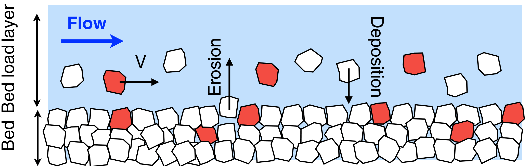
Figure 1Granular bed sheared by a steady and uniform flow. The bed is a mixture of marked (red) and unmarked (white) grains.

Download

Complemented with initial and boundary conditions, Eqs. (6) and (7) describe the evolution of the plume. In dimensionless form, they read

where $\widehat{t}$ = t∕τ_f and $\widehat{x}$ = x∕ℓ_f are dimensionless variables. For ease of notation, we drop the hat symbol in what follows.

A single parameter controls Eqs. (9) and (10): the ratio of surface densities α, which characterizes the average distance between grains in the bed load layer. Since the erosion–deposition model assumes independent particles, we can only expect it to be valid when moving particles are sufficiently far away from each other, which is when α is small or, equivalently, when the Shields parameter is near the threshold.

In the next section, we numerically solve Eqs. (9) and (10).

Laboratory measurements of bed load often use top-view images (Lajeunesse et al., 2017; Martin et al., 2012). Unless individual particles can be tracked, the tracers at rest are usually indistinguishable from those entrained by the flow. Separating the proportion of tracers in the moving layer, ϕ, from that on the bed surface, ψ, is practically impossible. Instead, top-view pictures show the total concentration of tracers:

Tracking sediment in rivers poses a similar problem. In general, one records the position of the tracers when the river stage is below the threshold of grain entrainment (Phillips and Jerolmack, 2014; Phillips et al., 2013). At the time of measurement, all tracers are therefore at rest. As a result, the proportion of mobile tracers vanishes (ϕ = 0), and the total concentration of tracers reads c = ψ∕(α + 1).

In summary, the proportions of mobile and static tracers, ϕ and ψ, naturally derive from mass balance (Eq. 2) and Eq. (3). However, their measurement proves difficult during active transport. On the other hand, experimental and field investigations provide the total concentration of tracers, c (Lajeunesse et al., 2017; Sayre and Hubbell, 1965). This quantity is conservative, as the total amount of tracers, M = ∫c dx, is preserved. In the following, we therefore focus on the concentration of tracers, c.

To study the evolution of the tracer concentration, we solve Eqs. (9) and (10) numerically using a finite-volume scheme. We then compute the tracer concentration using Eq. (11) (Fig. 2).

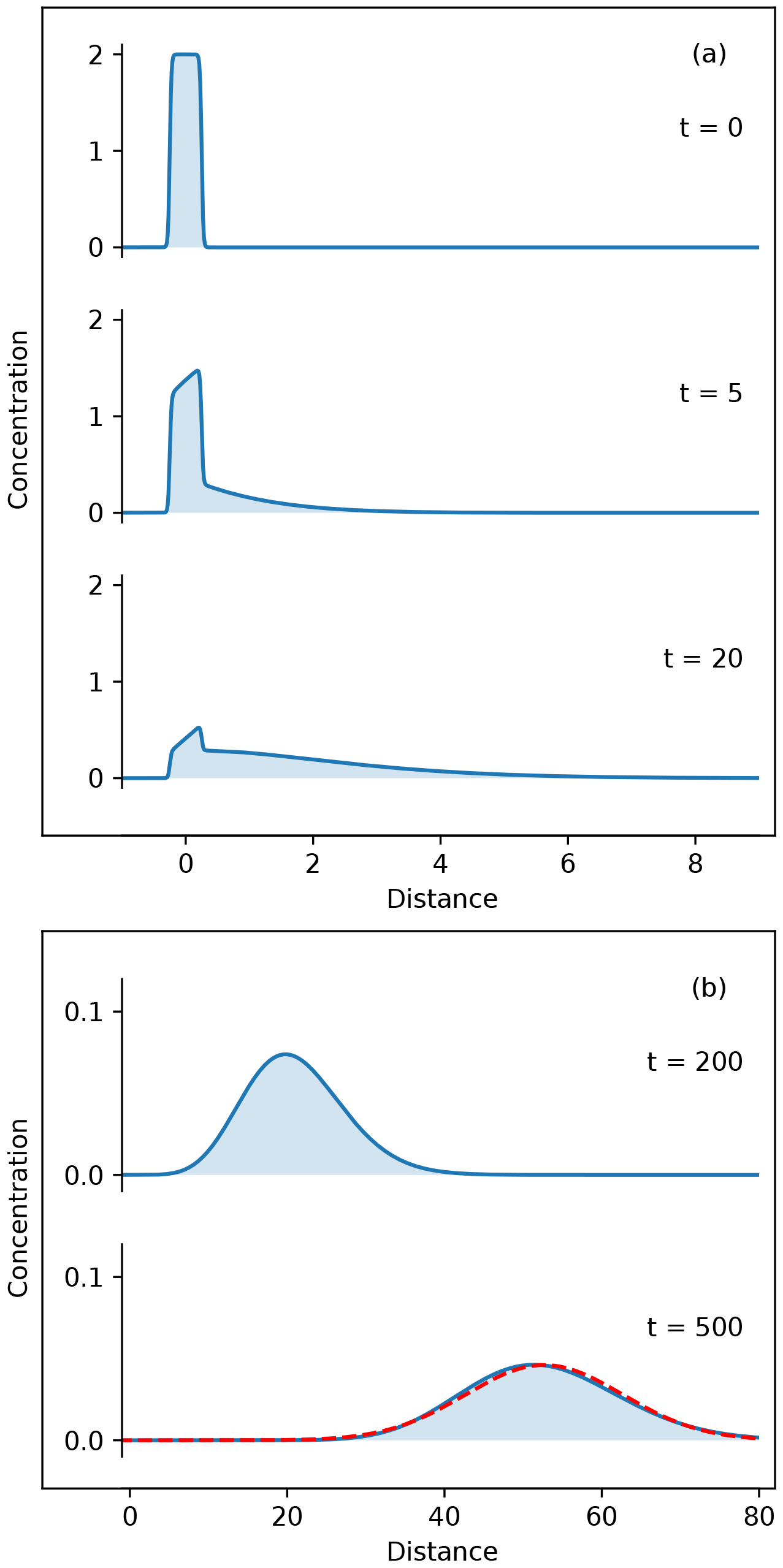
Figure 2Evolution of the tracer concentration (α = 0.1) obtained by numerically solving Eqs. (9) and (10). (a) Early entrainment regime. (b) Relaxation towards the diffusive regime. Tracers are initially at rest, forming a symmetric plume of length L = 0.5 and mass M = 1. The concentration profile asymptotically tends towards a Gaussian distribution (dotted red line).

Download

The early evolution of the plume depends on initial conditions. In most field experiments, tracers are deposited at the surface of the river bed when the flow stage is low and sediment is motionless (Phillips et al., 2013). During floods, the river discharge increases and the shear stress eventually exceeds the entrainment threshold, setting in motion some of the grains. The entrainment of particles strongly depends on the arrangement of the bed: grains highly exposed to the flow move first (Agudo and Wierschem, 2012; Charru et al., 2004; Turowski et al., 2011). Several authors find that the tracers they disposed on the bed are more mobile during the first flood than during later ones (Bradley and Tucker, 2012). During the later floods, tracers gradually get trapped in the bed, and their average mobility decreases. On the other hand, Phillips and Jerolmack (2014) find no special mobility during the first flood. In the absence of a clear scenario, we choose the simplest possible initial conditions and assume that initially all tracers belong to the static layer: ϕ(x, t = 0) = 0.

With these initial conditions, the evolution of the plume follows two distinct regimes. At early times, the flow gradually dislodges tracers from the bed and entrains them in the bed load layer. During this entrainment regime, only a small proportion of the tracers move. Consequently, the plume develops a thin tail in the downstream direction (Fig. 2a). The corresponding distribution of travel distances is strongly skewed towards the direction of propagation, a feature commonly observed in field experiments (Liébault et al., 2012; Phillips and Jerolmack, 2014).

With time, the plume moves downstream and spreads both upstream and downstream. As a result, the concentration rapidly decreases to small levels. The plume becomes gradually symmetrical and tends asymptotically towards a Gaussian distribution (Fig. 2b). This regime is reminiscent of classical diffusion.

To better illustrate this evolution, we introduce the mean position of the plume of tracers:

We also characterize its size with the variance,

and its symmetry with the skewness,

The evolution of these three moments is consistent with the existence of two asymptotic regimes (Fig. 3). At short timescales, the plume grows a thin tail downstream. This deformation causes the plume's skewness to increase as t⁴. During this regime, the average location of the plume increases as t² and its variance grows as t³. Although the variance increases nonlinearly with time, the exponent, 3, is too large for super-diffusion (Weeks and Swinney, 1998).

After a characteristic time of the order of τ ≈ τ_f, the skewness of the plume reaches a maximum (Fig. 3c). This corresponds to a drastic change in dynamics: the skewness starts decreasing as the plume becomes gradually more symmetrical. At long timescales, the plume of tracers advances at constant velocity and diffuses linearly with time (Fig. 3a and b). This regime, regardless of the value of α, corresponds to classical advection–diffusion.

Next, we establish the equivalence between diffusion and the long-time behavior of the tracers.

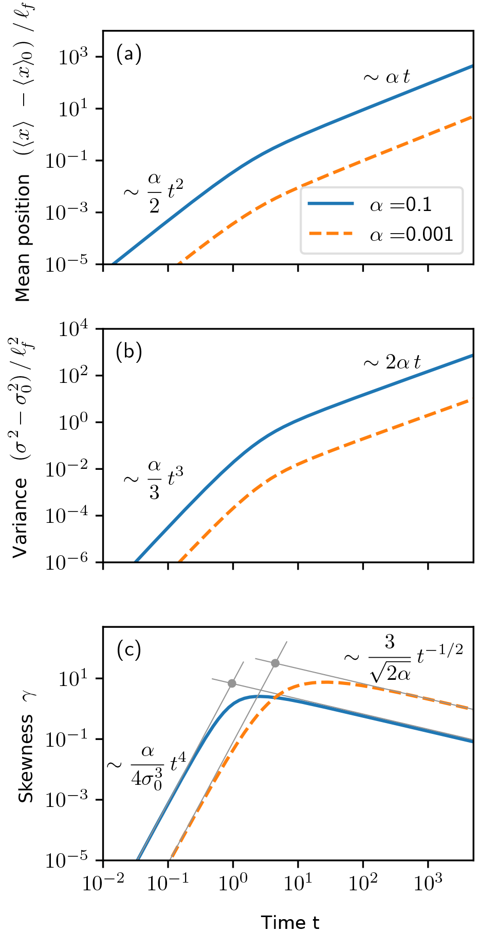
Figure 3(a) Position, (b) variance, and (c) skewness of a plume of tracers as a function of time for α = 0.1 and α = 0.001. We compute the evolution of these three quantities using Eqs. (28), (33), and (38). The results agree exactly with numerical simulations. The asymptotic regimes of the skewness are represented with grey lines. Their intersection provides an estimate of the duration of the entrainment regime (see Eq. 45).

Download

The diffusion at work in Eqs. (9) and (10) results from the continuous exchange of particles between the bed load layer, where particles travel at the constant velocity V, and the sediment bed, where particles are at rest. The velocity difference between the two layers gradually smears out the plume and spreads it in the flow direction. This process occurs in a variety of physical systems in which layers moving at different velocities exchange a passive tracer. A typical example is Taylor dispersion, whereby a passive tracer diffuses across a Poiseuille flow in a circular pipe (Taylor, 1953). The combination of shear rate and transverse molecular diffusion generates an effective diffusion in the flow direction. Other examples of effective diffusion include solute transport in porous media and chromatography (Van Genuchten and Wierenga, 1976).

To formally establish the equivalence between diffusion and the long-time behavior of the plume, we follow a reasoning similar to the one developed for chromatography (James et al., 2000). Equations (9) and (10) are equivalent to

where we introduce δ = ψ − ϕ, the difference between the proportion of tracers on the sediment bed and that in the bed load layer. Eventually, these proportions equilibrate each other. At long timescales, we therefore expect the solution to Eqs. (15) and (16) to relax towards steady state, for which δ is of order ϵ ≪ 1. Accordingly, we rewrite these two equations as

Introducing T = ϵt and X = ϵx and developing c and δ with respect to ϵ yields

at zeroth order and

at first order.

By multiplying Eq. (21) by ϵ and summing the result with Eq. (19), we finally get

At long timescales, the transport of the tracers follows the advection–diffusion equation (Eq. 22). We identify the advection velocity, U, which reads

Likewise, the diffusion coefficient reads

This asymptotic equivalence explains the advection–diffusion regime (Figs. 2 and 3).

We interpret this formal derivation as follows. In the reference frame of the plume, a tracer at rest on the bed moves backward, while a tracer entrained in the bed load layer moves forward. At long timescales, the proportions of tracers in each layer equilibrate. Consequently, the probability that a tracer will be entrained and move forward equals that of deposition. In the reference frame of the plume, the exchange of particles between the bed and the bed load layer is thus a Brownian motion driving the linear diffusion of the plume.

In the next section, we investigate the evolution of the location, the size, and the symmetry of the plume as it propagates downstream.

Concentration, defined as the number of tracers per unit of area, depends on the area over which it is measured. Its value is meaningful when the measurement area is much larger than the distance between particles and much smaller than the plume. During the entrainment regime, the plume develops a thin tail containing only a small proportion of tracers. Measuring the concentration profile during this regime is thus challenging. To our knowledge, only Sayre and Hubbell (1965) were able to measure consistent concentration profiles using radioactive sand. In practice, most field campaigns involve a limited number of tracers (900 at most) (Bradley, 2017; Bradley and Tucker, 2012; Liébault et al., 2012; Phillips and Jerolmack, 2014). It is thus more practical to consider integral quantities, such as the mean position of the plume 〈x〉, its variance σ², and its skewness γ.

Multiplying Eq. (15) by x and integrating over space provides the evolution equation for the mean position:

where

is the average difference between the proportion of tracers on the sediment bed and in the bed load layer. To solve Eq. (25), we need an equation for 〈δ〉. The latter is obtained by integrating Eq. (16) over space:

Equations (25) and (27) describe the downstream motion 〈x〉 of the plume. To solve them, we need to specify initial conditions. As discussed in Sect. 3, we consider all tracers to initially belong to the static layer, i.e., ϕ(x, t = 0) = 0. This condition and the conservation of mass, 〈c〉 = 1, provide initial conditions for 〈δ〉: 〈δ〉(t = 0) = α + 1. With this condition, Eqs. (25) and (27) integrate into

where 〈x〉₀ is the initial position of the plume.

We now focus on the variance of the plume. Multiplying Eq. (15) by x² and integrating over space yields the evolution equation for the second moment of the tracer distribution:

where

is the first moment of δ. To solve Eq. (29), we need an equation for this intermediate quantity. We obtain it by multiplying Eq. (16) by x and integrating over space:

At time t = 0, 〈xδ〉(t = 0) = (α + 1)〈x〉₀. Equations (29) and (31) with this initial condition provide the expression of the second moment of the tracer distribution:

where 〈x²〉₀ is the initial value of the second moment of the tracer distribution. We then deduce the variance of the plume from

We follow a similar procedure to derive the skewness of the plume. Multiplying Eq. (15) by x³ and integrating over space yields the evolution equation for the third moment of the tracer distribution:

where

is the second moment of δ. Multiplying Eq. (16) by x² and integrating over space provides the evolution equation for this intermediate quantity:

At time t = 0, 〈x²δ〉 = (α + 1)〈x²〉₀ and 〈x³〉 = 0. With these initial conditions, Eqs. (34) and (36) provide the expression of 〈x³〉:

from which we deduce the skewness of the plume as

Equations (28), (32), (33), (37), and (38) represent the evolution of the mean, the variance, and the skewness of the tracer distribution. They describe the migration, spreading, and symmetry of the plume. They do not require any assumption other than the ones of the model itself and agree exactly with numerical simulations (Fig. 3).

As discussed in Sect. 3, numerical simulations reveal a transient during which the tracers, initially at rest, are gradually set into motion by the flow (Fig. 3). During this entrainment regime, the plume continuously accelerates, spreads nonlinearly, and becomes increasingly asymmetrical. To characterize this regime, we expand Eqs. (28), (32), (33), (37), and (38) to leading order in time:

These three equations are consistent with our numerical simulations (Fig. 3).

Anomalous diffusion arises from heavy-tailed distributions of either the step length or the waiting time (Weeks and Swinney, 1998). The erosion–deposition model contains no such ingredient. Here the fast increase in the variance results from the exchange of particles between the sediment bed and the bed load layer at the beginning of the experiment. Over a time shorter than the flight duration τ_f, the tracers entrained by the flow do not settle back on the bed. They form a thin tail, which leaves the main body of the plume and moves downstream at the average particle velocity V (Fig. 2a). The plume therefore consists of a main body of virtually constant concentration, followed by a thin tail of length ∝Vt. Accordingly, we can split the integral that defines its mean position, Eq. (12), into two terms. The first one, obtained by integrating cx over the main body of the plume, yields the initial position of the plume 〈x〉₀. The second one, obtained by integrating cx over a tail of length Vt, scales as t². Summing these contributions yields Eq. (39). Similar reasonings yield Eqs. (40) and (41) for the variance and the skewness.

With time, the plume enters the diffusive regime. Its velocity and its spreading rate relax towards constants while its skewness decreases (Fig. 3). We derive the corresponding asymptotic behavior by expanding Eqs. (28), (32), (33), (37), and (38) in the limit of time being large:

The asymptotic regimes (Eqs. 42 and 43) are consistent with the expressions derived in Sect. 4.

The transition between the entrainment and the diffusive regime occurs when the skewness reaches its maximum value. Equating the skewness estimated from Eqs. (41) and (44) provides the approximate duration of the entrainment regime, τ. We find

which compares well with our numerical simulations (Fig. 3). The duration of the entrainment regime increases with the initial size of the plume and decreases with the intensity of sediment transport.

The asymptotic regimes (Eqs. 39, 40, 41, 42, 43, and 44) assume that sediment transport is in steady state. In the next section, we discuss the intermittency of bed load transport in natural streams.

Our description of the plume of tracers is based on the assumption that sediment transport is in steady state. This hypothesis is often satisfied in laboratory flumes (Lajeunesse et al., 2017). In a river, it may be met for up to a few days (Sayre and Hubbell, 1965). At longer timescales, however, most rivers alternate between low-flow stages during which sediment is immobile and floods during which bed particles are entrained downstream (Phillips and Jerolmack, 2016). Bed load transport is thus intermittent.

The intermittency of bed load transport influences the propagation of tracers in several ways. First of all, sediment transport during a flood modifies the structure of the bed (Lenzi et al., 2004; Turowski et al., 2009, 2011). As a result, the proportion of tracers in the bed load layer and in the bed, ϕ and ψ, likely change from one flood to the next. In a effort to address this question, P. Allemand and collaborators recently implemented the survey of a river located on Basse-Terre Island (Guadeloupe archipelago). Their preliminary observations reveal that the cobbles deposited at the end of a flood are the first entrained at the beginning of the next (P. Allemand, personal communication, 30 June 2017). Based on this observation, we speculate that a tracer belonging to the bed load layer at the end of a flood will still be part of the bed load layer at the beginning of the next one. Similarly, a tracer locked in the bed at the end of a flood will belong to the static layer at the beginning of the next one. In other words, we assume that tracers freeze between two floods.

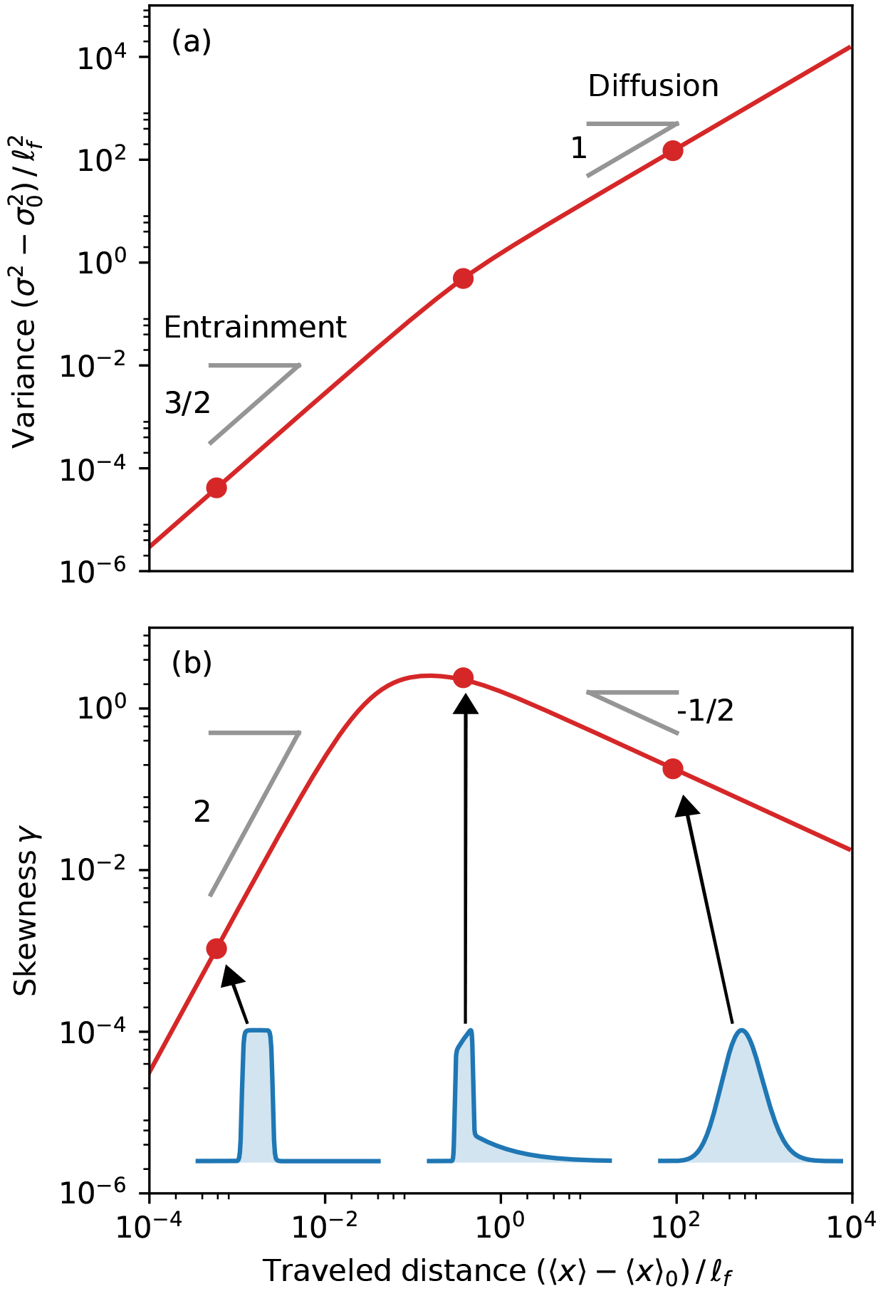
Figure 4(a) Variance and (b) skewness of a plume of tracers as a function of traveled distance (α = 0.1). These three quantities are calculated from Eqs. (28), (33), and (38). Inset: concentration profiles (blue) illustrating the shape of the plume during the entrainment regime (left), at the transition between the entrainment and the diffusive regime (center), and in the diffusive regime (right).

Download

If this assumption holds, the simplest way to account for bed load intermittency is to assume that the river alternates between two representative stages: (1) a low-flow stage during which tracers are immobile and (2) a flood stage characterized by a representative sediment flux q_s ∼ $\mathit{\alpha }V/d_{\mathrm{s}}^{\mathrm{2}}$ during which tracers propagate downstream (Paola et al., 1992; Phillips et al., 2013). Following this model, we may extrapolate our results to the field, provided we rescale time with respect to an intermittency factor I = T_e∕T, where T is the total duration of elapsed time, and T_e is the time during which sediments are effectively in motion (Paola et al., 1992; Parker et al., 1998; Phillips et al., 2013).

In practice, evaluating the intermittency factor requires continuous monitoring of the river discharge and a correct estimate of the entrainment threshold. Liébault et al. (2012), for instance, monitored the location of tracer cobbles deposited in the Bouinenc stream (France) during 2 years. Over this period, the motion of the tracers resulted from 55 floods for a total duration of 42 days. Sediments were thus in motion less than I = 12 % of the time.

Here, we suggest another way to circumvent the intermittency of sediment transport. Plotting the plume variance, (σ² − ${\mathit{\sigma }}_{\mathrm{0}}^{\mathrm{2}}$), and its skewness, γ, as a function of traveled distance, 〈x〉 − 〈x〉₀, eliminates time from the equations (Fig. 4). In this plot, the position of the plume acts as a proxy for the effective duration of sediment transport, T_e. The resulting curves are thus filtered from transport intermittency (Fig. 4).

The entrainment regime corresponds to small traveled distances. In this regime, both the size of the plume and its asymmetry increase with traveled distance (Fig. 4). Equations (39), (40), and (41) describe the early evolution of the plume. Eliminating time by combining them, we find the behavior of the plume for short traveled distances:

As discussed in Sect. 5, these scalings result from the gradual entrainment of the tracers that are initially trapped in the bed.

After the plume has traveled over a distance roughly equal to the flight length, its skewness reaches a maximum value and starts decreasing. This change in dynamics indicates the transition towards the diffusive regime. Equations (42), (43), and (44) provide the long-term behavior of the plume:

The linear increase in the variance with the distance traveled by the plume is the signature of standard diffusion (see Sect. 5).

Equating the skewness estimated from Eqs. (47) and (49) provides the position 〈x〉_max at which the skewness reaches its maximum:

The entrainment regime lasts until the plume has traveled over a distance comparable to its initial size, which is until 〈x〉 − 〈x〉₀ ∼ σ₀.

When expressed in terms of the distance traveled by the plume, the asymptotic regimes are insensitive to the intermittency of bed load transport. They are thus a robust test of our model and can help us interpret field data. Let us assume that a dataset records the evolution of a plume of tracers released in a river over a distance long enough to explore both the entrainment and the diffusive regime. During the diffusive regime, the skewness decreases with the traveled distance. A fit of the data with Eq. (49) yields the flight length, ℓ_f. Knowing the latter, we could use Eq. (47) to estimate the intensity of sediment transport, α, from the evolution of the skewness during the entrainment regime.

According to Sect. 5, the skewness reaches a maximum after a time τ_e (Eq. 45). Taking into account the intermittency of bed load transport in natural streams, we expect that this maximum is reached when

where I is the intermittency factor. Identifying this maximum in a field experiment thus yields the ratio τ_f ∕ I. Combining the latter with our estimates of the flight length, ℓ_f, and the intensity of sediment transport, α, should provide us with the average sediment transport rate in the river:

No data sets were used in this article.

The authors declare that they have no conflict of interest.