2.1 Utility of electromagnetic methods in coastal environments

Methods to ascertain the alongshore variability in framework geology, and to test long-range dependence, are difficult to implement and can be costly. Cores provide detailed point-wise geologic data; however, they do not provide laterally continuous subsurface information (Jol et al., 1996). Alternatively, geophysical techniques including seismic and GPR provide spatially continuous stratigraphic information (e.g., Buynevich et al., 2004; Neal, 2004; Nummedal and Swift, 1987; Tamura, 2012), but they are not ideally suited for LRD testing because the data combine depth and lateral information at a single acquisition point. Moreover, GPR signals attenuate rapidly in saltwater environments whereas seismic methods are labor-intensive and cumbersome. Conversely, terrain conductivity profiling is an easy-to-use alternative that has been used in coastal environments to investigate fundamental questions involving instrument performance characteristics (Delefortrie et al., 2014; Weymer et al., 2016), groundwater dynamics (Stewart, 1982; Fitterman and Stewart, 1986; Nobes, 1996; Swarzenski and Izbicki, 2009), and framework geology (Seijmonsbergen et al., 2004; Weymer et al., 2015a). Previous studies combining EMI with either GPR (Evans and Lizarralde, 2011) or coring (Seijmonsbergen et al., 2004) demonstrate the validity of EMI measurements as a means to quantify alongshore variations in the framework geology of coastlines.

In the alongshore direction, Seijmonsbergen et al. (2004) used a Geonics EM34^™ terrain conductivity meter crossing a former outlet of the Rhine River, Netherlands, to evaluate alongshore variations in subsurface lithology. The survey was conducted in an area that was previously characterized by drilling and these data were used to calibrate the σ_a measurements. The results from the study suggest that coastal sediments can be classified according to σ_a signature and that high σ_a values occur in areas where the underlying conductive layer is thick and close to the surface. Although Seijmonsbergen et al. (2004) propose that EMI surveys are a rapid, inexpensive method to investigate subsurface lithology, they also acknowledge that variations in salinity as a result of changing hydrologic conditions, storm activity, and/or tidal influence confound the geological interpretation and should be investigated in further detail (see Weymer et al., 2016).

The challenge on many barrier islands and protected national seashores is obtaining permission for extracting drill cores to validate geophysical surveys. At PAIS, numerous areas along the island are protected nesting sites for the endangered Kemp's ridley sea turtle and migratory birds while other areas comprise historic archeological sites with restricted access. Thus, coring is not allowed and only noninvasive techniques, such as EMI–GPR, are permitted.

2.2 Regional setting

North Padre Island is part of a large arcuate barrier island system located along the Texas Gulf of Mexico coastline. The island is one of 10 national seashores in the United States and is protected and managed by the National Park Service, a bureau of the Department of the Interior. PAIS is 129 km in length, and is an ideal setting for performing EMI surveys because there is minimal cultural noise to interfere with the σ_a signal, which as stated earlier we regard as a proxy for alongshore variations in framework geology (Fig. 1). Additionally, there are high-resolution elevation data available from a 2009 aerial lidar survey. The island is not dissected by inlets or navigation channels (excluding Mansfield Channel separating the North and South Padre islands) or modified by engineered structures (e.g., groynes, jetties) that often interfere with natural morphodynamic processes (see Talley et al., 2003). The above characteristics make the study area an exceptional location for investigating the relationships between large-scale framework geology and surface morphology.

As described in Weymer et al. (2015a; Fig. 3), locations of several paleo-channels were established by Fisk (1959) based on 3000 cores and seismic surveys. More than 100 boreholes were drilled to the top of the late Pleistocene surface (tens of meters of depth) providing sedimentological data for interpreting the depth and extent of the various paleo-channels. These cores were extracted ∼ 60 years ago, but the remnant Pleistocene and Holocene fluvial–deltaic features described in Fisk's study likely have not changed over decadal timescales.

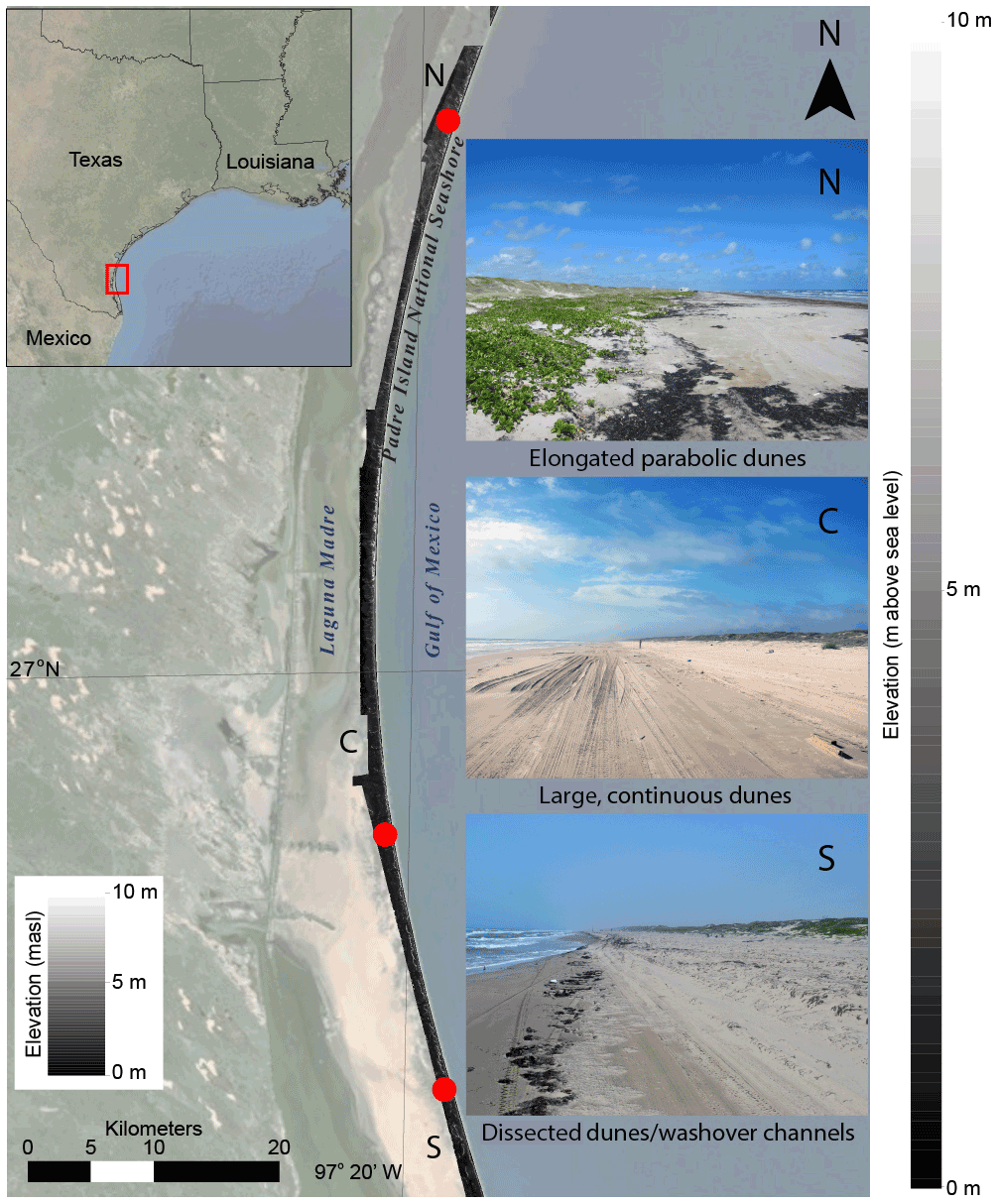
Figure 1Location map and DEM of the study area at Padre Island National Seashore (PAIS), Texas, United States. Elevations for the DEM are reported as meters above sea level (m a.s.l.). Approximate locations of field images (red dots) from the northern (N), central (C), and southern (S) regions of the island showing alongshore differences in beach–dune morphology. Note that views are facing south for the central and southern locations, and the northern location view is to the north. Images taken in October 2014.

Download

Geologic interpretations based on the Fisk (1959) data suggest that the thickness of the modern beach sands is ∼ 2–3 m, and they are underlain by Holocene shoreface sands and muds to a depth of ∼ 10–15 m (Brown and Macon, 1977; Fisk, 1959). The Holocene deposits lie upon a Pleistocene ravinement surface of fluvial–deltaic sands and muds and relict transgressive features. A network of buried valleys and paleo-channels in the central segment of the island, as interpreted by Fisk (1959), exhibits a dendritic, tributary pattern. The depths of the buried valleys inferred from seismic surveys range from ∼ 25 to 40 m (Brown and Macon, 1977). These channels have been suggested to have incised into the Pleistocene paleo-surface and became infilled with sands from relict Pleistocene dunes and fluvial sediments reworked by alongshore currents during the Holocene transgression (Weise and White, 1980). However, the location and cross-sectional area of each valley and paleo-channel alongshore is not well constrained. It is also possible that other channels exist other than those identified by Fisk (1959). As suggested in Weymer et al. (2015a), minima in the alongshore σ_a signal are spatially correlated with the locations of these previously identified geologic features. This observation provides an impetus for using EMI to map the known, and any previously unidentified, geologic features alongshore.

3.1 Field EMI and GPR surveys

Profiles of EMI σ_a responses are typically irregular and each datum represents a spatial averaging of the bulk subsurface electrical conductivity σ, which in turn is a function of a number of physical properties (e.g., porosity, lithology, water content, salinity). The “sensor footprint”, or subsurface volume over which the spatial averaging is performed, is dependent on the separation between the transmitter–receiver (TX–RX) coils (1.21 m in this study) and the transmitter frequency. The horizontal extent, or radius, of the footprint can be more or less than the step size between subsequent measurements along the profile. The sensor footprint determines the volume of ground that contributes to σ_a at each acquisition point, and as will be discussed later, the radius of the footprint has important implications for analyzing LRD. The footprint radius depends on frequency and ground conductivity, but is likely to be of the same order as, but slightly larger than, the intercoil spacing. Two different station spacings were used to examine the correlation structure of σ_a as a function of spatial scale. An island-scale alongshore survey of ∼ 100 km length was performed using a 10 m station spacing (station spacing ≫ footprint radius) such that each σ_a measurement was recorded over an independently sampled volume of ground. Additionally, a sequence of σ_a readings was collected at 1 m of spacing (station spacing < footprint radius) over a profile length of 10 km within the Fisk (1959) paleo-channel region of the island. This survey design allows for comparison of the long-range-dependent structure of the framework geology over several orders of magnitude (10⁰–10⁵ m).

The 100 km long alongshore EMI survey was performed during a series of three field campaigns, resulting in a total of 21 (each of length ∼ 4.5 km) segments that were collected during 9–12 October 2014, 15–16 November 2014, and 28 March 2015. The EMI σ_a profiles were stitched together by importing GPS coordinates from each measurement into ArcGIS^™ to create a single composite spatial data series. The positional accuracy recorded by a TDS Recon PDA equipped with a Holux^™ WAAS GPS module was found to be accurate within ∼ 1.5 m. To reduce the effect of instrument drift caused by temperature, battery, and other systematic variations through the acquisition interval, a drift correction was applied to each segment and the segments were then stitched together, following which a regional linear trend removal was applied to the composite dataset. An additional 10 km survey was performed along a segment of the same 100 km survey line in one day on 29 March 2015. This second composite data series consists of eight stitched segments.

The same multifrequency GSSI Profiler EMP-400^™ instrument was used for each segment. All transects were located in the back-beach environment ∼ 25 m inland from the mean tide level (MTL). This location was chosen to reduce the effect of changing groundwater conditions in response to nonlinear tidal forcing (see Weymer et al., 2016), which may be significant closer to the shoreline. As will be shown later, there is not a direct correlation between high tide and high σ_a values. Thus, we assume the tidal influence on the EMI signal can be neglected over the spatial scales of interest in the present study. Nevertheless, the duration and approximate tidal states of each survey were documented in order to compare with the EMI signal. Tidal data were accessed from NOAA's Tides and Currents database (NOAA, 2015b). Padre Island is microtidal and the mean tidal range within the study area is 0.38 m (NOAA, 2015a). A tidal signature in EMI signals may become more significant at other barrier islands with larger tidal ranges.

For all surveys, the EMI profiler was used in the same configuration and acquisition settings as described in Weymer et al. (2016). The transect locations were chosen to avoid the large topographic variations (see Santos et al., 2009) fronting the foredune ridge that can reduce the efficiency of data acquisition and influence the EMI signal. Measurements were made at a constant step size to simplify the data analysis; for example, ARIMA models require that data are taken at equal intervals (see Cimino et al., 1999). We choose herein to focus on data collected at 3 kHz, resulting in a depth of investigation (DOI) of ∼ 3.5–6.4 m over the range of conductivities found within the study area (Weymer et al., 2016; Table 1). Because the depth of the modern beach sands is ∼ 2–3 m or greater (see Brown and Macon, 1977; p. 56, Fig. 15), variations in the depth to shoreface sands and muds is assumed to be within the DOI of the profiler, which may not be captured at the higher frequencies also recorded by the sensor (i.e., 10 and 15 kHz) .

An 800 m GPR survey was performed on 12 August 2015 across one of the paleo-channels previously identified by Fisk (1959) located within the 10 km EMI survey for comparison with the σ_a measurements. We used a Sensors and Software pulseEKKO Pro^™ system for this purpose. A survey-grade GPS with a positional accuracy of 10 cm was used to match the locations and measurements between the EMI–GPR surveys. Data were acquired in reflection mode at a nominal frequency of 100 MHz with a standard antenna separation of 1 m and a step size of 0.5 m. The instrument settings resulted in a DOI of up to 15 m. Minimal processing was applied to the data and includes a dewow filter and migration (0.08 m ns⁻¹), followed by automatic gain control (AGC) gain (see Neal, 2004). The theory and operational principles of GPR are discussed in many places (e.g., Everett, 2013; Jol, 2008) and will not be reviewed here.

3.2 Geomorphometry

Topographic information was extracted from aerial lidar data that were collected by the U.S. Army Corps of Engineers (U.S. ACE) in 2009 as part of the West Texas Aerial Survey project to assess post-hurricane conditions of the beaches and barrier islands along the Texas coastline. This dataset is the most recent publicly available lidar survey of PAIS and it provides essentially complete coverage of the island. With the exception of Hurricane Harvey, which made landfall near Rockport, Texas, as a category 4 storm in late August, 2017, Padre Island has not been impacted by a hurricane since July 2008, when Hurricane Dolly struck South Padre Island as a category 1 storm (NOAA, 2015a). The timing of the lidar and EMI surveys in this study precede the impacts of Hurricane Harvey, and it is assumed that the surface morphology across the island at the spatial scales of interest (i.e., 10¹–10² km) did not change appreciably between 2009 and 2015.

A 1 m resolution DEM was created from 2009 lidar point clouds available from NOAA's Digital Coast (NOAA, 2017). The raw point cloud tiles were merged to produce a combined point cloud of the island within the park boundaries of PAIS. The point clouds were processed into a continuous DEM using the ordinary kriging algorithm in SAGA GIS, which is a freely available open-source software (http://www.saga-gis.org, last access: 13 January 2018), and subsequent terrain analysis was conducted using an automated approach involving the relative relief (RR) metric (Wernette et al., 2016). Several morphometrics including beach width, dune height, and island width were extracted from the DEM by averaging the RR values across window sizes of 21 m × 21 m, 23 m × 23 m, and 25 m × 25 m. The choice of window size is based on tacit a priori knowledge and observations of the geomorphology in the study area. A detailed description of the procedure for extracting each metric is provided in Wernette et al. (2016).

Each DEM series is paired with the σ_a profile by matching the GPS coordinates (latitude and longitude) recorded in the field by the EMI sensor. Cross-sectional elevation profiles oriented perpendicular to the shoreline were analyzed every 10 m (y coordinate) along the EMI profile to match the same 10 m sampling interval of the σ_a measurements. The terrain variations along each cross-shore profile are summed to calculate beach and island volume based on the elevation thresholds mentioned above. Dune volume is calculated by summing the pixel elevations starting at the dune toe, traversing the dune crest, and ending at the dune heel. In total, six DEM morphometrics were extracted as spatial data series to be paired with the EMI data, each with an identical sample size (n = 9694), which is sufficiently large for statistical ARIMA modeling.

3.3 Statistical methods

Although the procedures for generating the EMI and lidar datasets used in this study are different, the intended goal is the same: to produce spatial data series that contain similar numbers of observations for comparative analysis using a combination of signal processing and statistical modeling techniques. The resulting signals comprising each data series represent the spatial averaging of a geophysical (EMI) or geomorphological elevation variable that contains information about the important processes that form relationships between subsurface geologic features and island geomorphology that can be teased out by means of comparative analysis (Weymer et al., 2015a). Because we are interested in evaluating these connections at both small and large spatial scales, our first approach is to determine the autocorrelation function and Hurst coefficient (self-similarity parameter) H and hence verify whether the data series are characterized by short- and/or long-range memory (Beran, 1992; Taqqu et al., 1995). LRD occurs when the autocorrelation within a series, at large lags, tends to zero like a power function, and so slowly that the sums diverge (Doukhan et al., 2003). LRD is often observed in natural time series and is closely related to self-similarity, which is a special type of LRD.

The degree of LRD is related to the scaling exponent H of a self-similar process, where increasing H in the range 0.5 < H ≤ 1.0 indicates an increasing tendency towards such an effect (Taqqu, 2003). Large correlations at small lags can easily be detected by models with short memory (e.g., ARMA, Markov processes) (Beran, 1994). Conversely, when correlations at large lags slowly tend to zero like a power function, the data contain long-memory effects and either fractional Gaussian noise (fGn) or ARIMA models may be suitable (Taqqu et al., 1995). The R∕S statistic is the quotient of the range of values in a data series and the standard deviation (Beran, 1992, 1994; Hurst, 1951; Mandelbrot and Taqqu, 1979). When plotted on a log∕log plot, the resulting slope of the best-fit line gives an estimate of H, which is useful as a diagnostic tool for estimating the degree of LRD (see Beran, 1994).

It has been suggested that R∕S tends to give biased estimates of H, too low for H > 0.72 and too high for H < 0.72 (Bassingthwaigthe and Raymond, 1994), which was later confirmed by Malamud and Turcotte (1999). Empirical trend corrections to the estimates of H can be made by graphical interpolation, but are not applied here because of how the regression is performed. The R∕S analysis in this study was performed using signal analysis software AutoSignal^™ to identify whether a given signal is distinguishable from a random, white noise process and, if so, whether the given signal contains LRD. The H value is calculated by an inverse variance-weighted linear least-squares curve fit using the logarithms of the R∕S and the number of observations, which provides greater accuracy than other programs that compute the Hurst coefficient.

Two of the simplest statistical time series models that can account for LRD are fGn and ARIMA. In the former case, fGn and its “parent” fractional Brownian motion (fBm) are used to evaluate stationary and nonstationary fractal signals, respectively (see Eke et al., 2000; Everett and Weiss, 2002). Both fGn and fBm are governed by two parameters: variance σ² and the scaling parameter, H (Eke et al., 2000). A more comprehensive class of time series models that has a similar capability to detect long-range structure is ARIMA. Because fGn and fBm models have only two parameters, it is not possible to model the short-range components. Additional parameters in ARIMA models are designed to handle the short-range component of the signal, as discussed by Taqqu et al. (1995) and others. Because the EMI data series presumably contain both short-range and long-range effects, we chose to use ARIMA as the analyzing technique.

ARIMA models are used across a wide range of disciplines in geoscience and have broad applicability for understanding the statistical structure of a given data series as it is related to some physical phenomenon (see Beran, 1992, 1994; Box and Jenkins, 1970; Cimino et al., 1999; Granger and Joyeux, 1980; Hosking, 1981; Taqqu et al., 1995). For example, Cimino et al. (1999) apply R∕S analysis, ARIMA, and neural network analysis to different geological datasets including tree ring data, Sr isotope data of Phanerozoic seawater samples, and El Niño phenomena. The authors show that their statistical approach enables (1) recognition of qualitative changes within a given dataset, (2) evaluation of the scale (in)dependency of increments, (3) characterization of random processes that describe the evolution of the data, and (4) recognition of cycles embedded within the data series. In the soil sciences, Alemi et al. (1988) use ARIMA and Kriging to model the spatial variation in clay-cover thickness of a 78 km² area in northeastern Iran and demonstrate that ARIMA modeling can adequately describe the nature of the spatial variations. ARIMA models have also been used to model periodicity of major extinction events in the geologic past (Kitchell and Pena, 1984).

In all these studies, the statistical ARIMA model of a given data series is defined by three terms ($p,d,q$), where p and q indicate the order of the autoregressive (AR) and moving average (MA) components, respectively, and d represents a differencing or integration term (I) that is related to LRD. The AR element, p, represents the effects of adjacent observations and the MA element, q, represents the effects on the process of nearby random shocks (Cimino et al., 1999; De Jong and Penzer, 1998). However, in the present study our series are reversible spatial series that can be generated, and are identical, with either forward or backward acquisition, unlike a time series. Both p and q parameters are restricted to integer values (e.g., 0, 1, 2), whereas the integration parameter, d, represents potentially long-range structure in the data. The differencing term d is normally evaluated before p and q to identify whether the process is stationary (i.e., constant mean and σ²). If the series is nonstationary, it is differenced to remove either linear (d = 1) or quadratic (d = 2) trends, thereby making the mean of the series stationary and invertible (Cimino et al., 1999), thus allowing determination of the ARMA p and q parameters.

Here, we adopt the definitions of an ARMA (p,q), and ARIMA ($p,d,q$) process following the work of Beran (1994). Let p and q be integers, where the corresponding polynomials are defined as

It is important to note that all solutions of ϕ(x₀)=0 and ψ(x)=0 are assumed to lie outside the unit circle. Additionally, let ${\mathit{ϵ}}_t(t=\mathrm{1},\mathrm{2},\mathrm{\dots })$ be independent, and identically distributed normal variables with zero variance ${\mathit{\sigma }}_{\mathit{ϵ}}^{\mathrm{2}}$ such that an ARMA (p,q) process is defined by the stationary solution of

where B is the backward shift operator $B{X}_t=X_{t-\mathrm{1}},B^{\mathrm{2}}{X}_t=X_{t-\mathrm{1}},\mathrm{\dots }$ and, specifically, the differences can be expressed in terms of B as $X_t-X_{t-\mathrm{1}}=(\mathrm{1}-B)X_t,(X_t-X_{t-\mathrm{1}})-(X_{t-\mathrm{1}}-X_{t-\mathrm{2}})=(\mathrm{1}-B{)}^{\mathrm{2}}{X}_t\mathrm{\dots }$ Alternatively, an ARIMA ($p,d,q$) process X_t is formally defined as

where Eq. (3) holds for a dth difference (1−B)^dX_t.

As mentioned previously, a more general form of ARIMA ($p,d,q$) is the fractional ARIMA process, or FARIMA, where the differencing term d is allowed to take on fractional values. If d is a non-integer value for some −0.5 < d < 0.5 and X_t is a stationary process as indicated by Eq.(3), then the model by definition is called a FARIMA process where d values in the range 0 < d < 0.5 are of particular interest herein because geophysically relevant LRD occurs for 0 < d < 0.5, whereas d > 0.5 means that the process is nonstationary but nonintegrable (Beran, 1994; Hosking, 1981). A special case of a FARIMA process explored in the current study is ARIMA (0d0), also known as fractionally differenced white noise (Hosking, 1981), which is defined by Beran (1994) and others as

For 0 < d < 0.5, the ARIMA (0d0) process is a stationary process with long-range structure and is useful for modeling LRD. As shown later, different values of the d parameter provide further insight into the type of causative physical processes that generate each data series. When d < 0.5, the series X_t is stationary, which has an infinite MA representation that highlights long-range trends or cycles in the data. Conversely, when d > −0.5, the series X_t is invertible and has an infinite AR representation (see Hosking, 1981). When −0.5 < d < 0, the stationary, and invertible, ARIMA (0d0) process is dominated by short-range effects and is anti-persistent. When d=0, the ARIMA (000) process is white noise, with zero correlations and a constant spectral density. Identification of an appropriate model is accomplished by finding small values of elements $p,d,q$ (usually between 0 and 2) that accurately fit the most significant patterns in the data series. When a value of an element is 0, that element is not needed. For example, if d=0 the series does not contain a significant long-range component, whereas if $p=q=\mathrm{0}$, the model does not exhibit significant short-range effects. If $p,d,q\ne \mathrm{0}$, the model contains a combination of both short- and long-memory effects.

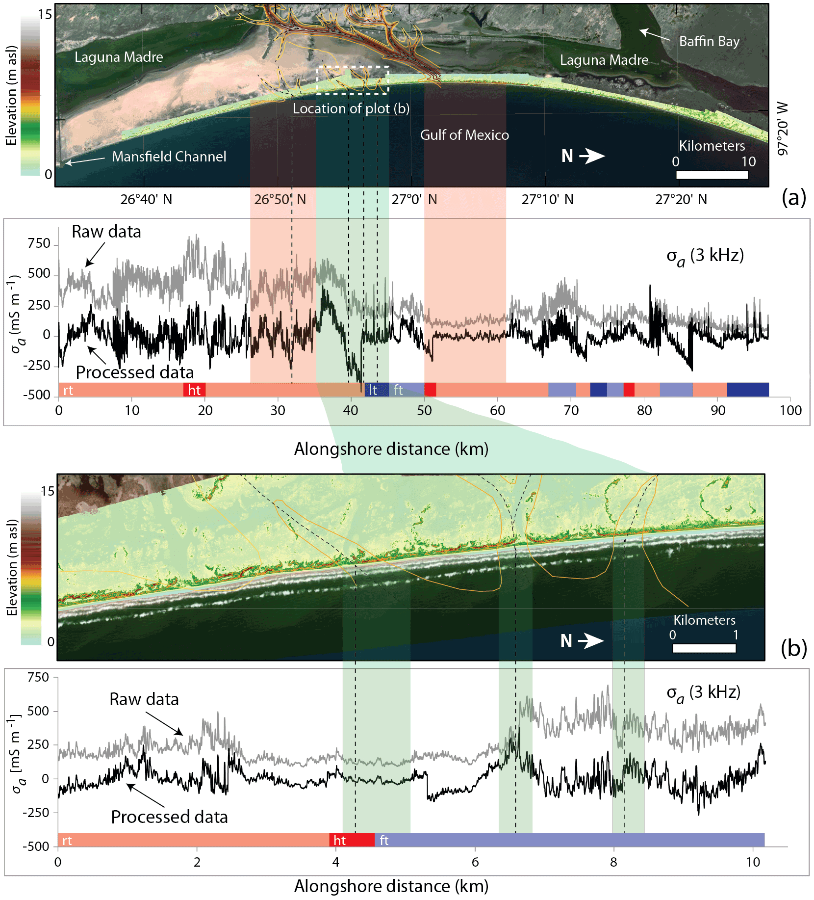
Figure 2The 100 km (a) and 10 km (b) alongshore EMI surveys showing DEMs of the study area and previously identified paleo-channel region by Fisk (1959). Channels are highlighted in red and green, where the green region indicates the location of the 10 km survey. The 25 ft (7.6 m) contour intervals are highlighted with depths increasing from yellow to red and the center of the channels are represented by the black-dotted lines. For each survey, raw σ_a and zero-mean drift-corrected EMI responses are shown in gray and black, respectively. Tidal conditions during each EMI acquisition segment are shown below each panel. Low (lt) and falling tides (ft) are indicated by blue and light blue shades, respectively. High (ht) and rising tides (rt) are highlighted in red and light red, respectively.

Download

4.1 Spatial data series

4.1.1 EMI and GPR surveys

The unprocessed (raw) EMI σ_a responses show a high degree of variability along the island. High-amplitude responses within the EMI signal generally exhibit a higher degree of variability (multiplicative noise) compared to the low-amplitude responses. Higher σ_a readings correspond to a small sensor footprint and have enhanced sensitivity to small-scale near-surface heterogeneities (see Guillemoteau and Tronicke, 2015). Low σ_a readings suggest the sensor is probing greater depths and averaging over a larger footprint. In that case, the effect of fine-scale heterogeneities that contribute to signal variability is suppressed.

The 10 km alongshore survey is located within an inferred paleo-channel region (Fisk, 1959), providing some a priori geologic constraints for understanding the variability within the EMI signal (Fig. 2b). Here, the sample size is n=10 176, permitting a quantitative comparison with the 100 km long data series since they contain a similar number of observations. Unlike the 100 km survey, successive footprints of the sensor at each subsequent measurement point overlap along the 10 km survey. The overlap enables a fine-scale characterization of the underlying geological structure because the separation between the TX and RX coils (1.21 m), a good lower-bound approximation of the footprint, is greater than the step size (1 m).

Figure 3Comparison of EMI σ_a responses from the 100 km survey with 100 MHz GPR data within one of the Fisk (1959) paleo-channels. The 800 m segment (A–A^′) crosses a smaller stream within the network of paleo-channels in the central zone of PAIS. The DOI of the 3 kHz EMI responses is outlined by the red box on the lower GPR radargram and the interpretation of the channel base (ravinement surface) is highlighted in yellow.

Download

The overall trend in σ_a for the 10 km survey is comparable to that of the 100 km survey, where regions characterized by high- and low-amplitude signals correspond to regions of high and low variability, respectively, implying that multiplicative noise persists independently of station spacing. The decrease in σ_a that persists between ∼ 2.5 and 6 km along the profile (Fig. 2b) coincides in location with two paleo-channels, whereas a sharp reduction in σ_a is observed at ∼ 8.2 km in close proximity to a smaller channel. Most of the known paleo-channels are located within the 10 km transect and likely contain resistive infill sands that should generate lower and relatively consistent σ_a readings (Weymer et al., 2015a). The low σ_a signal caused by the sand indirectly indicates valley incision since it is diagnostic of a thicker sand section, relatively unaffected by the underlying conductive layers. Thus, it is reasonable to assume that reduced variability in the signal is related to the framework geology within the paleo-channels, which we now compare with a GPR profile.

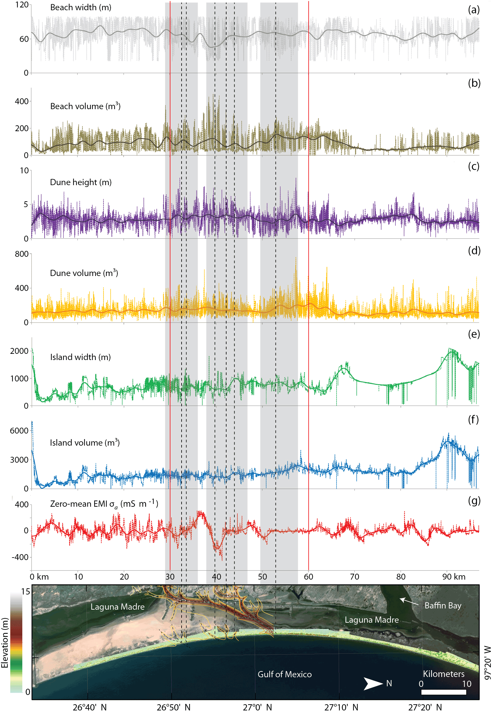
Figure 4DEM metrics extracted from aerial lidar data. The sampling interval (step size) for each data series is 10 m and the coordinates are matched with each EMI acquisition point. Each panel corresponds to (a) beach width, (b) beach volume, (c) dune height, (d) dune volume, (e) island width, (f) island volume, and (g) EMI σ_a. The island is divided into three zones (red vertical lines) roughly indicating the locations within and outside the known paleo-channel region. A Savitzky–Golay smoothing filter was applied to all data series (lidar and EMI) using a moving window of n=250 to highlight the large-scale patterns in each signal.

Download

To corroborate the capability of the EMI data to respond to the variable subsurface geology, an 800 m GPR survey confirms the location of a previously identified paleo-channel (Fisk, 1959) at ∼ 5–10 m depth (Fig. 3). A continuous undulating reflector from ∼ 150 to 800 m along the profile is interpreted to be the surface mapped by Fisk (1959), who documented a paleo-channel at this location with a depth of ∼ 8 m. Although the paleo-surface is within the detection limits of the GPR, it is likely that the DOI of the EMI data (∼ 3–6 m) is not large enough to probe continuously along the contact between the more conductive ravinement surface and the more resistive infill sands. Along the transect at shallower depths highlighted by the red box in the lower radargram (Fig. 3), low EMI σ_a values correspond to fine stratifications in the GPR section, which is common for beach sands with little clay content that are not saline-saturated. The EMI highs between ∼ 450 and 530 m coincide with parts of the GPR section that do not have the fine stratification and this may indicate the presence of clay or saline water. Here, the high conductivity zone for both the GPR and EMI is located within a recovering washover channel overlying the paleo-channel that is evident in the satellite imagery in the upper-left panel of Fig. 3. The overwash deposits consisting of a mix of sand and more finely grained backbarrier sediments likely mask the EMI sensors' ability to probe greater depths. Nonetheless, the high-conductivity zone represents a smaller ∼ 100 m segment within the ∼ 500 m wide paleo-channel, suggesting that variations in the EMI responses outside this zone are directly related to variations in the framework geology imaged by GPR.

4.1.2 Lidar-derived DEM morphometrics

The lidar-derived elevation data series along the 100 km transect are presented in Fig. 4. Each data series is shown with respect to the areal DEM of the study area where the approximate locations of each closely spaced paleo-channel are highlighted in gray. This visualization allows a qualitative analysis of the spatial relationships among paleo-channels, subsurface information encoded in the σ_a signal, and surface morphology over the entire length of the barrier island.

The morphology of the beach–dune system, as well as island width, changes substantially from north to south. In the paleo-channel region, beach width decreases in the central channel (∼ 37–42 km) and is more variable outside this region. Beach width generally increases towards the northern section of the island. The volume of the beach tends to be lowest in the northern zone, varies considerably in the central part of the island, then stabilizes and gradually decreases towards the south. These zones correspond to the southern (0–30 km), central (30–60 km), and northern (60–100 km) sections of the island. Alongshore dune heights are generally greater in the south, become slightly more variable in the paleo-channel region, and decrease in the north except for the area adjacent to Baffin Bay. Dune volume is lowest in the northern section, intermittently increases in the central zone, and slightly decreases towards the south. The island is considerably narrower between Mansfield Channel and Baffin Bay (see Fig. 2a), increasing in width in the northern zone; island volume follows a similar trend. Overall, σ_a values are lower northward of the paleo-channel region compared to the southern zone where σ_a increases substantially. However, the lowest σ_a values are located within the region of paleo-channels inferred by Fisk (1959), supporting previous findings in the study area by Weymer et al. (2015a) and Wernette et al. (2018) that suggest a potential geologic control on alongshore geomorphic features.

Each spatial data series (Fig. 4a–g) represents a different superposition of effects caused by physical processes operating across a wide range of temporal and length scales (Weymer et al., 2015a). Short-range fluctuations represent small-scale heterogeneities, whereas long-range components capture variations in each metric at broader length scales. There is a high degree of variability within each signal that is directly related to the geological and geomorphological structure along the island. Within and outside the paleo-channel region, general associations between EMI σ_a responses and DEM metrics are visually subtle, motivating the statistics we now show with ARIMA modeling. To conduct the ARIMA analysis, we chose to divide the island into three zones based on the location of the known paleo-channels. As will be discussed later, the tripartite zonation allows for a quantitative analysis of LRD at three spatial scales (regional, intermediate, local) within and outside the area containing paleo-channels. It is important to note, however, that the framework geology is likely to exhibit LRD regardless of the length-scale over which it is observed.

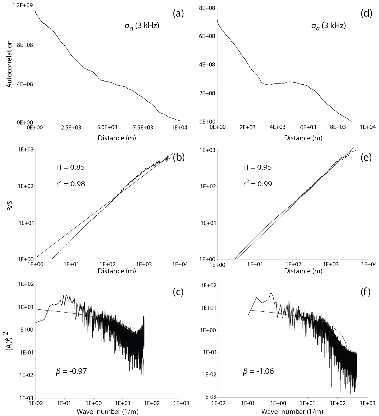
Figure 5Autocorrelations of σ_a for the 100 km (a) and 10 km EMI surveys (d). R∕S analysis for the 100 km (b) and 10 km surveys (e). PSD plots for the 100 km (c) and 10 km surveys (f).

Download

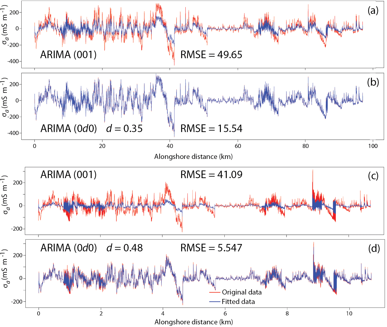
Figure 6Examples of the worst-fit (a, c) and best-fit (b, d) ARIMA models for the 100 and 10 km EMI surveys. Model results are shown for the processed (drift-corrected) σ_a data. Residuals (RMSE) listed for each model give the standard deviation of the model prediction error. For each plot, original data are in red and fitted (model) data are in blue.

Download

4.2 Tests for LRD

4.3 ARIMA statistical modeling of EMI

The results of the tests described in Sect. 4.2.1 for estimating the self-similarity parameter H and the slope of the PSD function suggest that both EMI data series, and by inference the underlying framework geology, exhibit LRD. The goal of our analysis using ARIMA is to estimate the p, d, and q terms representing the order, respectively, of AR, integrated (I), and MA contributions to the signal (Box and Jenkins, 1970) to quantify free vs. forced behavior along the island. For the analysis, the “arfima” and “forecast” statistical packages in R were used to fit a family of ARIMA ($p,d,q$) models to the EMI σ_a data and island morphometrics (Hyndman, 2015; Hyndman and Khandakar, 2008; Veenstra, 2013). Results of 10 realizations drawn from a family of ARIMA ($p,d,q$) models and their residuals (RMSE) are presented in Table 1. The worst fit (ARIMA 001) models are shown for the 100 and 10 km (Fig. 6a, c) surveys. The best fit (ARIMA 0d0) models for both the 100 and 10 km surveys are shown in Fig. 6b and d, respectively. For this analysis, the tests include different combinations of $p,d,$ and q that model either short-range: ARIMA (100; 001; 101; 202; 303; 404; 505), long-range: ARIMA (010; 0d0), or composite short- and long-range processes: ARIMA (111). It is important to note that AR and MA are only appropriate for short-memory processes since they involve only near-neighbor values to explain the current value, whereas the integration (the I term in ARIMA) models long-memory effects because it involves distant values. Note that ARIMA was developed for one-way time series, in which the arrow of time advances in only one direction, but in the current study we are using it for spatial series that are reversible. Different realizations of each ARIMA ($p,d,q$) data series were evaluated, enabling physical interpretations of LRD at regional, intermediate, and local spatial scales. Determining the best-fitting model is achieved by comparing the residual score, or RMSE, of each predicted data series relative to the observed data series, where lower RMSE values indicate a better fit (Table 1).

Table 1Comparison of residuals (RMSE) of each ARIMA model for the 100 and 10 km EMI surveys.

Download Print Version | Download XLSX

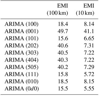
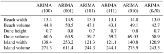
Table 2Comparison of residuals (RMSE) of each ARIMA model for all spatial data series. Note that the residuals for each DEM metric correspond to the analysis performed at the regional scale (i.e., 100 km).

Download Print Version | Download XLSX

Based on the residuals and visual inspection of each realization (Fig. 6), two observations are apparent: (1) both EMI data series are most accurately modeled by an ARIMA (0d0) process with non-integer d, and (2) the mismatch between the data and their model fit is considerably lower for the 10 km survey compared to the 100 km survey. The first observation suggests that the data are most appropriately modeled by a FARIMA process, i.e., a fractional integration that is stationary (0 < d < 0.5) and has long-range dependence (see Hosking, 1981). This implies that spatial variations in framework geology at the broadest scales dominate the EMI signal and that small-scale fluctuations in σ_a caused, for example, by changing hydrological conditions over brief time intervals less than the overall data acquisition interval, or fine-scale lithological variations less than a few station spacings, are not as statistically significant. Regarding the second observation, the results suggest that a small station spacing (i.e., 1 m) is preferred to accurately model both short- and long-range contributions within the signal because large station spacings cannot capture short-range information. The model for the 10 km survey fits better because both p (AR) and q (MA) components increase with a smaller step size since successive volumes of sampled subsurface overlap. On the contrary, the sensor footprint is considerably smaller than the station spacing (10 m) for the 100 km survey. Each σ_a measurement in that case records an independent volume of ground, yet the dataset still exhibits LRD, albeit not to the same degree as in the 10 km survey.

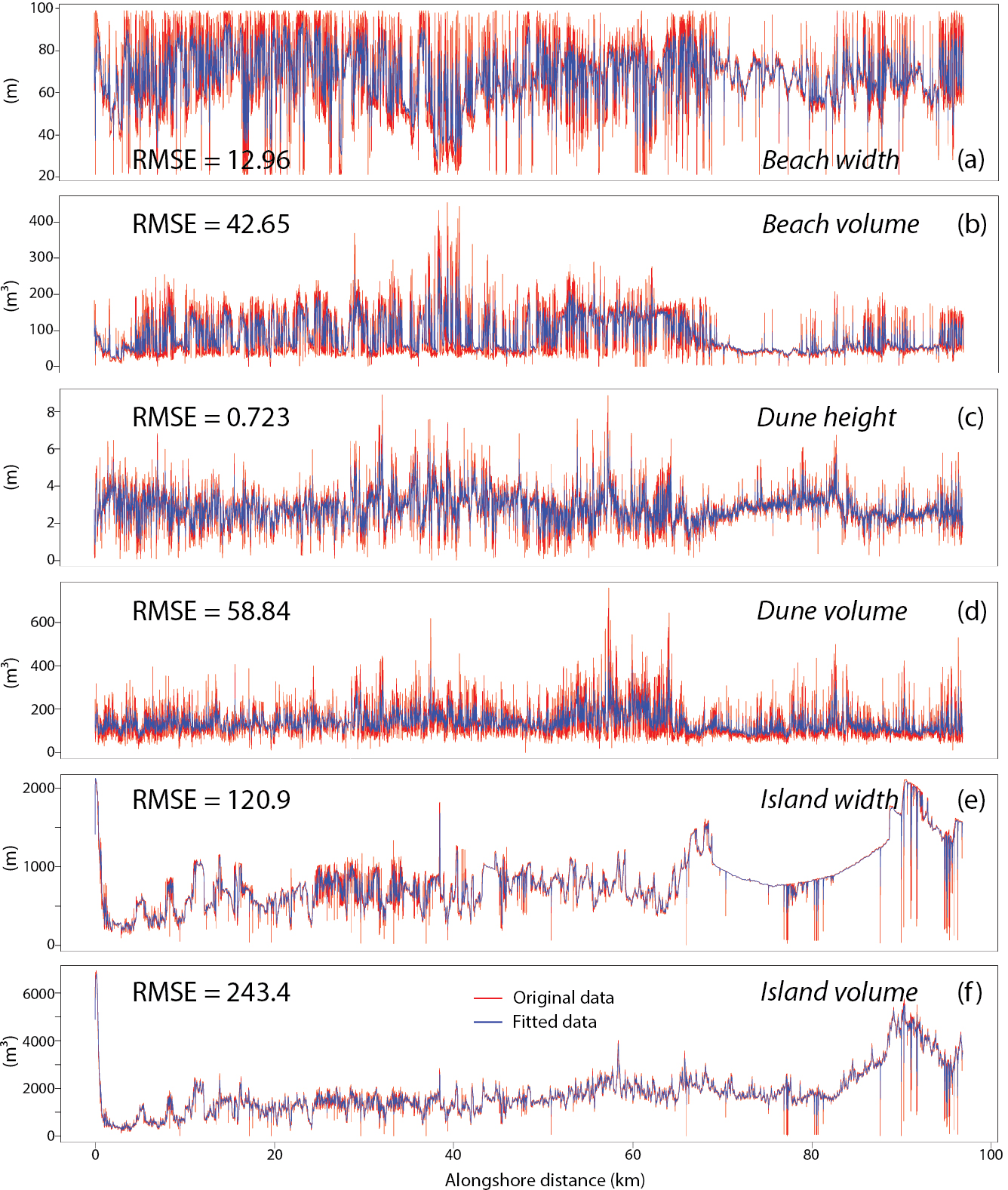
Figure 7Example of the best fit ARIMA (0d0) models for each lidar-derived DEM metric: (a) beach width, (b) beach volume, (c) dune height, (d) dune volume, (e) island width, and (f) island volume.

Download

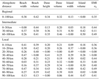
Table 3Summary table showing the computed d parameters that most appropriately model each ARIMA (0d0) iteration (i.e., lowest RMSE).

Download Print Version | Download XLSX

4.4 ARIMA statistical modeling of island metrics compared with EMI

A sequence of ARIMA ($p,d,q$) models was also evaluated for the elevation morphometrics series to find best fits to the data. The analysis comprised a total of 36 model tests (Table 2). The RMSE values reveal that (1) all data series are best fit by an ARIMA (0d0) process with fractional d, i.e., a FARIMA process; (2) the ARIMA models, in general, more accurately fit the EMI data than the DEM morphometric data likely because the morphology is controlled by more than the framework geology alone; and (3) in all cases, the poorest fit to each series is the ARIMA (001) or MA process. This, in turn, means that the differencing parameter d is the most significant parameter amongst p, d, and q. It is important to note that different values of d were computed based on the best fit of each FARIMA model to the real data. A graphical representation of the FARIMA-modeled data series for each DEM metric is shown in Fig. 7, allowing a visual inspection of how well the models fit the observed data. Because each data series has its own characteristic amplitude and variability, it is not possible to compare RMSE among tests without normalization. The variance within each data series can differ by several orders of magnitude.

Instead of normalizing the data, a fundamentally different approach is to compare the EMI σ_ad values with respect to each metric at regional, intermediate, and local scales (Table 3). Higher positive d values indicate a stronger tendency towards LRD. According to Hosking (1981), {x_t} is called an ARIMA (0d0) process and is of particular interest in modeling LRD as d approaches 0.5 because in such cases the correlations and partial correlations of {x_t} are all positive and decay slowly towards zero as the lag increases, while the spectral density of {x_t} is concentrated at low frequencies. It is reasonable to assume that the degree of LRD may change over smaller intermediate and/or local scales, which implies a breakdown of self-similarity. For a self-similar signal, d is a global parameter that does not depend on which segment of the series is analyzed. In other words, the d values should be the same at all scales for a self-similar structure.

The results of the FARIMA analysis at the intermediate scale vary considerably within each zone of the barrier island (north, central, south) and for each spatial data series (Table 3). In the southern zone (0–30 km), EMI σ_a and beach volume have the strongest LRD (d=0.44), whereas the other metrics exhibit weak LRD (ranging from d ∼ 0 to 0.2), which may be characterized approximately as a white noise process. Within the paleo-channel region (30–60 km), all of the island metrics show a moderate to strong tendency towards LRD (0.3 ≤ d ≤ 4.2); however, the EMI signal does not (d=0.11). In the northern zone (60–100 km) all data series contain moderate to strong LRD with the exception of beach and island width.

A FARIMA analysis was also conducted at the local scale by dividing the island into 10 km segments, starting at the southern zone (0–10 km) and ending at the northern zone of the island (90–100 km). A total of 70 FARIMA model realizations were evaluated and the resulting d values demonstrate that the EMI data segments show a stronger presence of LRD (d > 0.4) within the paleo-channels (30–60 km) and further to the north (60–80 km) in close proximity to the ancestral outlet of Baffin Bay. These findings indicate that there may be local and/or intermediate geologic controls along different parts of the island, but that the framework geology dominates island metrics at the regional scale.