the Creative Commons Attribution 4.0 License.
the Creative Commons Attribution 4.0 License.
 | 22 Jun 2018
How concave are river channels?
Fiona J. Clubb
Boris Gailleton
Martin D. Hurst
For over a century, geomorphologists have attempted to unravel information about landscape evolution, and processes that drive it, using river profiles. Many studies have combined new topographic datasets with theoretical models of channel incision to infer erosion rates, identify rock types with different resistance to erosion, and detect potential regions of tectonic activity. The most common metric used to analyse river profile geometry is channel steepness, or ks. However, the calculation of channel steepness requires the normalisation of channel gradient by drainage area. This normalisation requires a power law exponent that is referred to as the channel concavity index. Despite the concavity index being crucial in determining channel steepness, it is challenging to constrain. In this contribution, we compare both slope–area methods for calculating the concavity index and methods based on integrating drainage area along the length of the channel, using so-called “chi” (χ) analysis. We present a new χ-based method which directly compares χ values of tributary nodes to those on the main stem; this method allows us to constrain the concavity index in transient landscapes without assuming a linear relationship between χ and elevation. Patterns of the concavity index have been linked to the ratio of the area and slope exponents of the stream power incision model (m∕n); we therefore construct simple numerical models obeying detachment-limited stream power and test the different methods against simulations with imposed m and n. We find that χ-based methods are better than slope–area methods at reproducing imposed m∕n ratios when our numerical landscapes are subject to either transient uplift or spatially varying uplift and fluvial erodibility. We also test our methods on several real landscapes, including sites with both lithological and structural heterogeneity, to provide examples of the methods' performance and limitations. These methods are made available in a new software package so that other workers can explore how the concavity index varies across diverse landscapes, with the aim to improve our understanding of the physics behind bedrock channel incision.
- Article
(6248 KB) - Full-text XML
-
Supplement
(5826 KB) - BibTeX
- EndNote


Geomorphologists have been interested in understanding controls on the steepness of river channels for centuries. In his seminal “Report on the Henry Mountains”, Gilbert (1877) remarked that “We have already seen that erosion is favoured by declivity. Where the declivity is great the agents of erosion are powerful; where it is small they are weak; where there is no declivity they are powerless” (p. 114). Following Gilbert's pioneering observations of landscape form, many authors have attempted to quantify how topographic gradients (or declivities) relate to erosion rates. Landscape erosion rates are thought to respond to tectonic uplift (Hack, 1960). Therefore, extracting erosion rate proxies from topographic data provides novel opportunities for identifying regions of tectonic activity (Cyr et al., 2010; Lague and Davy, 2003; Seeber and Gornitz, 1983; Snyder et al., 2000; Wobus et al., 2006a), and may even be able to highlight potentially active faults (Kirby and Whipple, 2012). Analysing channel networks is particularly important for detecting the signature of external forcings from the shape of the topography, as fluvial networks set the boundary conditions for their adjacent hillslopes, therefore acting as the mechanism by which climatic and tectonic signals are transmitted to the rest of the landscape (Burbank et al., 1996; Hurst et al., 2013; Whipple, 2004; Whipple and Tucker, 1999).
Channels do not yield such information easily, however. Any observer of rivers or mountains will note that headwater channels tend to be steeper than channels downstream. Declining gradients along the length of the channel lead to river longitudinal profiles that tend to be concave up. Therefore, the gradient of a channel cannot be related to erosion rates in isolation; some normalising procedure must be performed. Over a century ago, Shaler (1899) postulated that as channels gain drainage area their slopes would decline, hindering their ability to erode. Authors such as Hack (1957), Morisawa (1962), and Flint (1974) expanded upon this idea in the early 20th century by quantifying the relationship between slope and drainage area, often used as a proxy for discharge. Flint (1974) found that channel gradient appeared to systematically decline downstream in a trend that could be described by a power law:
where θ is referred to as the concavity index since it describes how concave a profile is; the higher the value, the more rapidly a channel's gradient decreases downstream. Note that the term “concavity” is sometimes applied to river long profiles (Conway et al., 2015; Demoulin, 1998; Roy and Sinha, 2018), so most studies refer to θ, derived from slope–area data, as the “concavity index” (Kirby and Whipple, 2012). The term ks is called the steepness index, as it sets the overall gradient of the channel. If we take the logarithm of both sides of Eq. (1), we find a linear relationship in log[S]–log[A] space with a slope of θ and an intercept (the value of log[S], where log[A] = 0) of log[ks]:
A number of studies (DiBiase et al., 2010; Harel et al., 2016; Mandal et al., 2015; Ouimet et al., 2009; Scherler et al., 2014) have demonstrated that ks is positively correlated with erosion rate, mirroring the predictions of Gilbert (1877) over a century earlier. Many authors have used channel steepness to examine fluvial response to climate, lithology, and tectonics (Cyr et al., 2010; DiBiase et al., 2010; Flint, 1974; Harkins et al., 2007; Kirby and Whipple, 2001, 2012; Kobor and Roering, 2004; Lague and Davy, 2003; Snyder et al., 2000; Tarboton et al., 1989; Vanacker et al., 2015; Wobus et al., 2006a).
The noise inherent in S–A analysis prompted Leigh Royden and colleagues to develop a method that compares the elevations of channel profiles, rather than slope (Royden et al., 2000). We can modify the Royden et al. (2000) approach to integrate Eq. (1), since S = dz∕dx where z is elevation and x is distance along the channel (Whipple et al., 2017), resulting in
where A0 is a reference drainage area, introduced to non-dimensionalise the area term within the integral in Eq. (3). We can then define a longitudinal coordinate, χ:
χ has dimensions of length and is defined such that at any point in the channel
Equation (5) shows that steepness of the channel (ks) is related to the slope of the transformed channel in χ–elevation space. In both Eqs. (2) and (5), the numerical value of ks depends on the value chosen for the concavity index, θ. In order to compare the steepness of channels in basins of different sizes, a reference concavity index is typically chosen (θref), which is then used to extract a normalised channel steepness from the data (Wobus et al., 2006a):
where the subscript i is a data point. This data point often represents channel quantities that are smoothed; see discussion below.
1.1 Choosing a concavity index to extract channel steepness
The choice of the reference concavity index is important in determining the relative ksn values amongst different sections in the channel network, which we illustrate in Fig. 1. This figure depicts hypothetical slope–area data, which appear to lie along a linear trend in slope–area space. Choosing a reference concavity index based on a regression through these data will result in the entire channel network having similar values of ksn. Based on the data in Fig. 1, there is no evidence that the correct concavity index is anything other than the one represented by the linear fit through the data. However, these hypothetical data are in fact based on numerical simulations, presented in Sect. 3, in which we simulated a higher uplift rate in the core of the mountain range. The correct concavity index is therefore lower than that indicated by the log[S]–log[A] data, and instead the data show a strong spatial trend in channel steepness (interpretation 2 in Fig. 1). The simplest interpretation based on log[S]–log[A] data alone would have been entirely incorrect. This situation is analogous to the one described by Kirby and Whipple (2001), where downstream reductions in uplift rates in the Siwalik Hills of India and Nepal resulted in elevated apparent concavities. Conversely, if a single reference concavity index is chosen in an area with changing concavity indices, then spurious patterns in ksn may arise (Gasparini and Whipple, 2014). These examples highlight that selecting the correct concavity index is crucial if we are to correctly interpret channel steepness data.
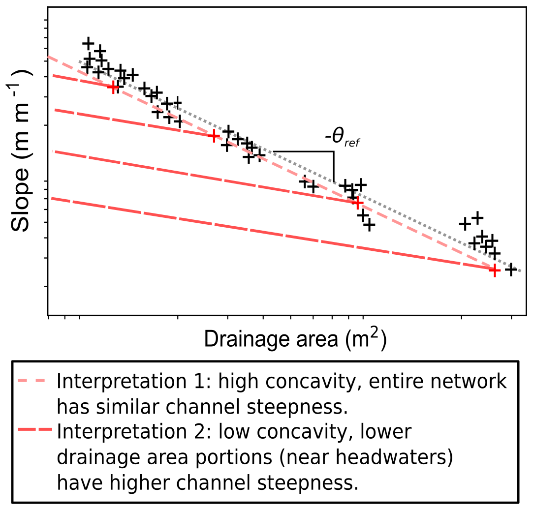
Figure 1Sketch illustrating the effect of choosing different reference concavities. The data can be well fitted with a single regression, suggesting that all parts of the channel network have similar values of ksn (interpretation 1). However, if a lower θref is chosen, the ksn values will be systematically higher for channels at lower drainage area (interpretation 2). This sketch is based on data from a numerical simulation where the latter situation has been imposed via higher uplift rates in the core of the mountain range, showing the potential for incorrect concavities to be extracted from slope–area data alone.
Extracting a reliable reference concavity indices from slope–area data on real landscapes is challenging: topographic data can be noisy, leading to a wide range of channel gradients for small changes in drainage area. The branching nature of river networks also results in large discontinuities in drainage areas where tributaries meet, resulting in significant data gaps in S–A space (Fig. 2). Wobus et al. (2006a) made recommendations for preprocessing of slope–area data that are still used in many studies. First, the digital elevation model (DEM) is smoothed (although with improved DEMs this is now rare), then topographic gradient is measured over either a fixed reach length or a fixed drop in elevation (Wobus et al., 2006a, recommends the latter), and then the data are averaged in logarithmically spaced bins. More recently, authors have proposed alternative channel smoothing strategies (Aiken and Brierley, 2013; Schwanghart and Scherler, 2017); all these methods use some form of smoothing and averaging.
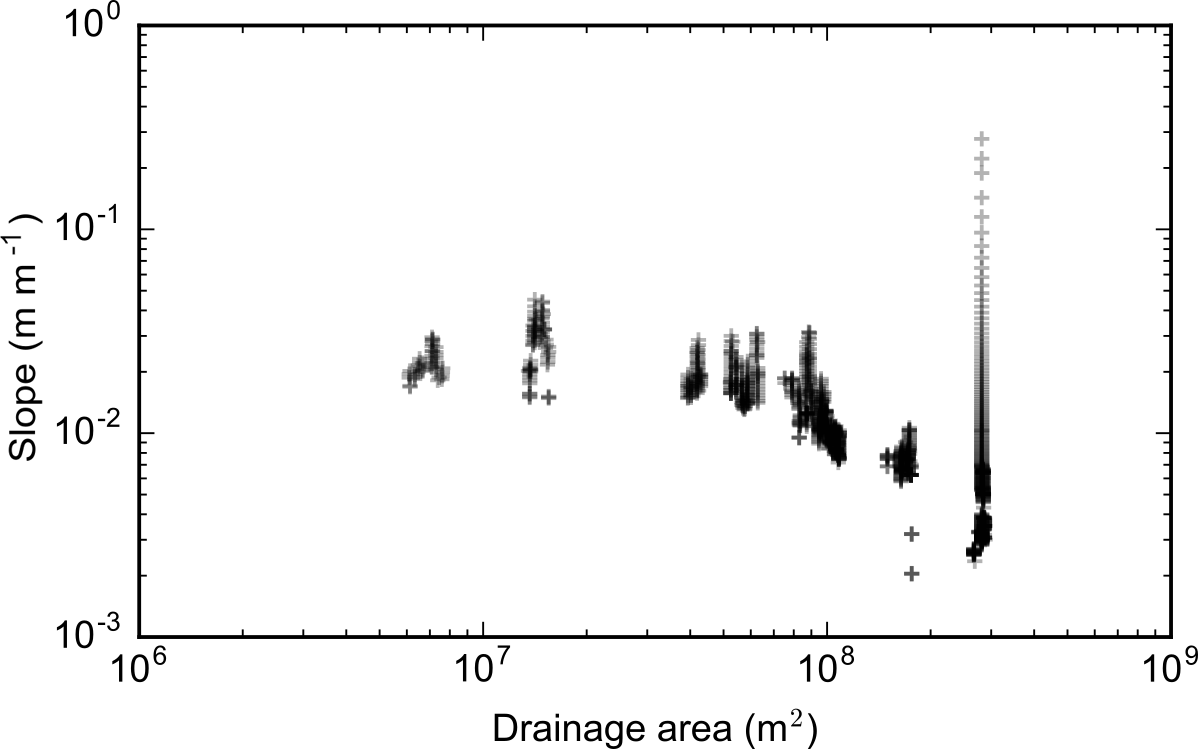
Figure 2A typical slope–area plot. This example is from a basin near Xi'an, China, with an outlet at approximately 34∘26′23.9 N, 109∘23′13.4 E. The data are taken from only the trunk channel. The slope–area data typically contain gaps due to tributary junctions, as well as wide ranges in slope for the reaches between junctions due to topographic noise inherent in deriving slope values. The result is a high degree of scatter in the data. These data are produced by averaging slope values over a fixed vertical interval of 20 m.
In order to circumvent these problems with S–A analysis, many authors have since used the integral approach (Eq. 5) to analyse channel concavity indices. This method also aims to normalise river profiles for their drainage area, but rather than comparing slope to area, it integrates area along channel length (Perron and Royden, 2013; Royden et al., 2000). Perron and Royden (2013) showed that the concavity index could be extracted from a channel by selecting the value of θref that results in the most linear channel profile in χ–elevation space. However, if there are sections of the channel with different ksn values, this will hinder our ability to extract the θref value, as it is not appropriate to fit a single line throughout the entire profile (Mudd et al., 2014). Mudd et al. (2014) introduced a method to statistically determine the most likely concavity index by computing the best-fit series of linear segments using an algorithm that balanced fit of the data against overparameterisation using the Akaike information criterion (Akaike, 1974). This method, however, requires a number of input parameters and also performs computationally expensive segmentation on the χ–elevation data prior to calculating the concavity index (Mudd et al., 2014).
Perron and Royden (2013) suggested a second independent means to calculate the concavity index, which does not assume linearity of the profiles in χ–elevation space and may therefore be used in transient landscapes. This method is instead based on searching for collinearity of tributaries with the main stem channel (Mudd et al., 2014; Perron and Royden, 2013), and has since been used as a basis for other techniques that aim to minimise some quantitative description of scatter between tributaries and the trunk channel Goren et al. (2014); Hergarten et al. (2016).
Although the collinearity test does not assume any linearity of profiles in χ–elevation space, it does rely on the assumption that points in the channel network with the same value of χ will have the same elevation. Perron and Royden (2013) noted that this will hold true if transient erosion signals propagate vertically through the network at a constant rate, which has been predicted by some theoretical models of fluvial incision (Wobus et al., 2006b). Royden and Perron (2013) went on to demonstrate that changes in erosion rates in channel networks would lead to distinct segments that migrate upstream, which they termed “slope patches”, where the local ks reflects local erosion rate. However, here, we wish to avoid basing our formulation on any theoretical models of fluvial incision, as this introduces assumptions regarding bedrock erosion processes. Y. Wang et al. (2017) highlighted that slope–area analysis could be used to complement integral analysis where concavity indices might vary spatially, since slope–area is agnostic with regard to these incision processes, but also found that integral-based analyses have lower uncertainties than slope–area analysis. Therefore, here, we use simple geometric relationships of knickpoint propagation to relate the collinearity test to channel concavity indices without relying on theoretical models of fluvial incision, as set out in Sect. 1.2.
1.2 Connecting the concavity index to collinearity
Playfair (1802) noted that tributary valleys tended to join the principal valley at a common elevation, suggesting that, at their outlets, the tributary streams must lower at the same rate as the principal streams into which they drain. Therefore, any change in incision rate on the main stem channel will be transmitted to the upstream tributaries. Using simple geometric relationships, Niemann et al. (2001) showed that a knickpoint should migrate upstream with a horizontal celerity (Ceh, in length per time) of
where S1 is the channel slope prior to disturbance, S2 is the channel slope after disturbance (e.g. due to a change in incision rate E), and ΔE is the difference between the incision rate before and after disturbance (which can be equated to uplift rates U1 and U2 in units of length per time, ). Wobus et al. (2006b) simply inserted Eq. (1) into Eq. (7) so that the horizontal celerity is simply a function of drainage area, assuming that the concavity index is independent of rock uplift rate:
Noting that vertical celerity is simply the horizontal celerity multiplied by the local slope after disturbance S2, Wobus et al. (2006b) showed that the vertical celerity (Cev) was not a function of drainage area:
Thus, if we assume spatially homogeneous uplift and constant erodibility (i.e. channels with the same slope and drainage area erode at the same rate), then the vertical celerity propagating up the principal stream and all tributaries will be a constant. Equation (9) is derived from purely geometric relationships, suggesting that collinearity can be used to estimate the concavity index without assuming any theoretical models of fluvial incision under the assumption that the incision process will result in local slope–area relationships reflecting Eq. (1).
In this study, we revisit commonly used methods for estimating the concavity index using both slope–area analysis and collinearity methods based on integral analysis. Our objective is to determine the strengths and weaknesses of established methods alongside several new methods developed for this study, as well as to quantify the uncertainties in the concavity index. We present these methods in an open-source software package that can be used to constrain concavity indices across multiple landscapes. This information may give insight into the physical processes responsible for channel incision into bedrock, which are as yet poorly understood.
2.1 Slope–area analysis
For slope–area analysis, in this paper, we forgo initial smoothing of the DEM and use a fixed elevation drop along a D8 drainage pathway implemented using the network extraction algorithm of Braun and Willett (2013). We calculate the best-fit concavity indices using two different methods: (i) concavity indices extracted from all slope–area (S–A) data (i.e. no logarithmic bins, every tributary) and (ii) concavity indices of contiguous channel profile segments with consistent S–A scaling within the log-binned S–A data of the trunk stream, calculated using the statistical segmentation algorithm described in Mudd et al. (2014). We report the different extracted concavity indices and their uncertainties in the results below.
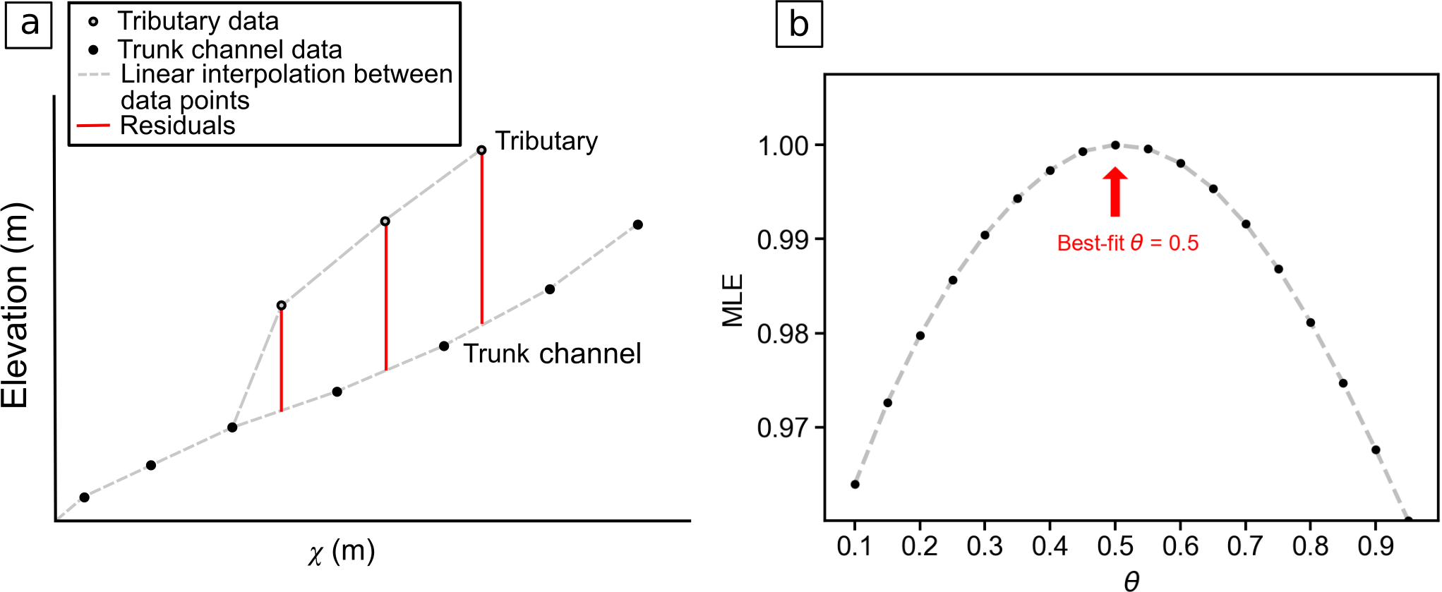
Figure 3Sketch illustrating the methodology of the χ method using all profile data. In panel (a), the χ profiles of both the trunk channel and a tributary are shown. We take the χ coordinate of the nodes on the tributary channel and then project them onto a linear fit of the trunk channel to determine the residuals between tributary and trunk channel. We do this for all nodes and for all concavity indices. For each concavity index, the residuals are then used to calculate a maximum likelihood estimator (MLE), which varies as a function of the concavity index (panel b). The highest value of MLE is used to select the likely θ.
2.2 Methods for calculating collinearity using integral analysis
Here, we present two new methods of identifying collinear tributaries in χ–elevation space in order to constrain the best-fit concavity indices from fluvial profiles. Rather than fitting segments to the profiles, which is computationally expensive, we directly compare all the elevation data of the tributaries in each drainage basin to the main stem. This is not completely straightforward, however: because the χ coordinate integrates area and channel distance, it is very unlikely that a pixel on a tributary channel shares a χ coordinate with any pixel on the main stem. Instead, for every tributary pixel, we compare the tributary elevation with an elevation on the main stem at the same χ computed with a linear fit between the two pixels with the nearest χ coordinates (Fig. 3). We then calculate a maximum likelihood estimator (MLE) for each tributary. The MLE is calculated with
where N is the number of nodes in the tributary, ri is the calculated residual between the elevation of tributary node i and the linear regression of elevation on the main stem, and σ is a scaling factor. If ri is 0 for all nodes, then MLE = 1 (i.e. MLE varies between 0 and 1, with 1 being the maximum possible likelihood).
For a given drainage basin, we can multiply the MLE for each tributary to get the total MLE for the basin, and we can do this for a range of concavity indices to calculate the most likely value of θ. Because Eq. (10) is a product of negative exponentials, the value of the MLE will decrease as N increases, and in large datasets this results in MLE values below the smallest number that can be computed, meaning that in large datasets MLE values can often be reported as zero. To counter this effect, we increase σ until all tributaries have non-zero MLE values. As σ is simply a scaling factor, this does not affect which concavity index is calculated as the most likely value once all tributaries have non-zero MLEs (see the Supplement).
There are two disadvantages to using Eq. (10) on all points in the channel network. Firstly, because the MLE is calculated as a product of exponential functions, each data point will reduce the MLE, and so tributaries will influence MLE in proportion to their length. Secondly, because we use all data, we cannot estimate uncertainty when computing the most likely concavity index. Therefore, we apply a second method to the χ–elevation data that mitigates these two shortcomings by bootstrap sampling the data. This method evaluates a fixed number of discrete points on each tributary, but the points are selected randomly and this random selection is done iteratively, building up a population of MLE values for each concavity index.
For each iteration of the bootstrap method, we create a template of points in χ space, measured from the confluence of each tributary from the trunk channel (Fig. 4). We start by selecting a maximum value of χ upstream of the tributary junction, and then separate this space into NBS nodes. We create evenly spaced bins between the maximum value of χ in the template, and then in each iteration randomly select one point in each bin. Using this template on each tributary, we calculate the residuals between the tributary and the trunk channel using Eq. (10). If, for a given tributary, a point in the template is located beyond the end of the tributary, then the point is excluded from the calculation of MLE. Figure 4 provides a schematic visualisation of this method.
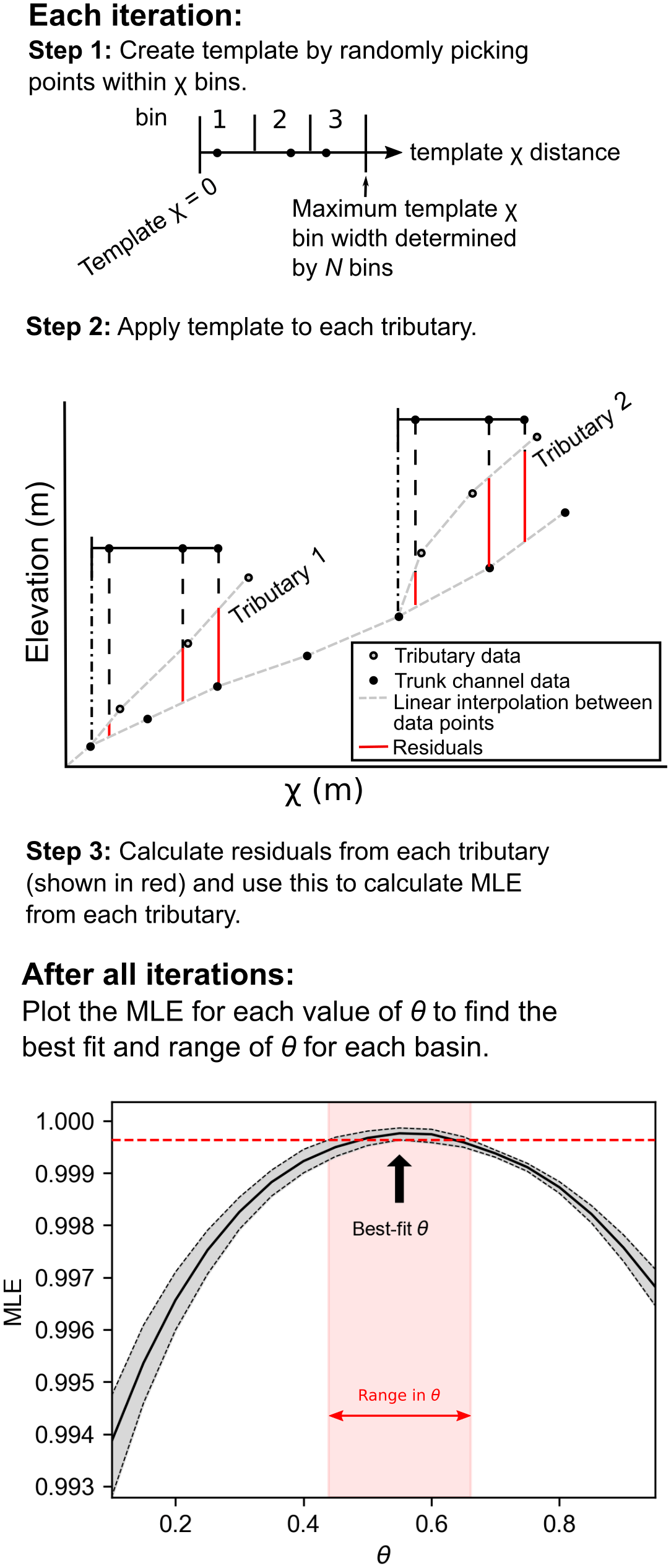
Figure 4Sketch showing how we compute residuals for our χ bootstrap method of determining the maximum likelihood estimator (MLE) of θ, and then use the uncertainty in MLE values to compute the uncertainty in θ.
We repeat these calculations over many iterations, and for each concavity index we compute the median MLE, the minimum and maximum MLEs, and the first and third quartile MLEs. We approximate the uncertainty range by first taking the most likely concavity index (having highest median MLE value amongst all concavity indices tested). We then find the span of concavity indices whose third quartile MLE values exceed the first quartile MLE value of the most likely concavity indices (Fig. 4).
One complication of using collinearity to calculate the most likely concavity index is that occasionally one may find a hanging tributary (Crosby et al., 2007; Wobus et al., 2006b), which could occur for a variety of reasons, such as the presence of geologic structures or lithologic variability. A hanging tributary can skew the overall MLE values in a basin, so in each basin we test the MLE and RMSE values in each tributary for outliers and iteratively remove these outlying tributaries, testing for the most likely concavity index on each iteration. However, we find that eliminating outlying tributaries has a minimal effect on the calculated concavity index. The other primary complication is that one must assume a concavity index prior to performing the χ transformation (Eq. 4), and thus slope–area analysis may be more suited to detecting changes in concavity within basins (Y. Wang et al., 2017). We suggest here an alternative approach of calculating concavity using χ methods in many small basins to look for any systematic changes. Before we can perform such analyses, however, we must constrain our confidence in estimates of the concavity index.
We also implement a disorder statistic (Goren et al., 2014; Hergarten et al., 2016; Shelef et al., 2018) that aims to quantify differences in the χ–elevation patterns between tributaries and the trunk channel. Here, we follow the method of Hergarten et al. (2016). The disorder statistic is calculated by first taking the χ–elevation pairs of every point in the channel network, ordered by increasing elevation. We calculate the sum:
where the subscript s, i represents the ith χ coordinate that has been sorted by its elevation. The sum, S, is minimal if elevation and χ are related monotonically. However, it scales with the absolute values of χ, which are sensitive to the concavity index (see Eq. 4), so following Hergarten et al. (2016), we scale the disorder metric, D, by the maximum value of χ in the tributary network (χmax):
The disorder metric relies on the use of all the data in a tributary network, meaning that only one value of D can be calculated for each basin. Therefore, we cannot estimate the uncertainty in concavity index using this statistic alone. Furthermore, the random sampling approach we take with the previous χ methods is not appropriate, as skipping nodes in the χ–elevation sequence will lead to large values of S and substantially increase the disorder metric. We therefore employ a bootstrap approach based on the analysis of entire tributaries within each basin. First, we find every combination of three tributaries plus the trunk stream in the basin. For each combination, we then iterate through a range of concavity indices and calculate the disorder metric. This allows us to find the concavity index that minimises the disorder metric for each combination, resulting in a population of best-fit concavities, from which we calculate the median and interquartile range.
In real landscapes, we can only approximate the concavity index based on topography. However, we can create simulations where we fix a known concavity index and see if our methods reproduce this value. To do this, we rely on simple simulations driven by the general form of the stream power incision model, first proposed by Howard and Kerby (1983):
where E is the long-term fluvial incision rate, A is the upstream drainage area, S is the channel gradient, K is the erodibility coefficient, which is a measure of the efficiency of the incision process, and m and n are exponents. A number of variations of this equation are possible: some authors have proposed, for example, modifications that involve erosion thresholds (Tucker and Bras, 2000) or modulation by sediment fluxes (Sklar and Dietrich, 1998). However, Gasparini and Brandon (2011) showed that many of the modified versions of Eq. (13) could be captured simply by modifying the exponents m and n.
We have chosen this model because it can be related to the concavity index and therefore can be used to test the different methods under idealised conditions. We can relate the stream power incision model to Eq. (1) by rearranging Eq. (13) to solve for channel slope and relating it to local erosion rate, E:
Comparing Eqs. (1) and (14) reveals that the ratio between area and slope exponents in the stream power incision model, m∕n, is therefore equivalent to θ from Eq. (1). The channel steepness index, ks, is related to erosion rate by
The stream power incision model also makes predictions about how tectonic uplift can be translated into local erosion rates (Whipple and Tucker, 1999), and the predicted relationship between the channel steepness index and uplift has been exploited by a number of studies to identify areas of tectonic activity (Kirby and Whipple, 2012; Kirby et al., 2003; Wobus et al., 2006a). Furthermore, many workers have used the framework of the stream power incision model to extract uplift histories (Fox et al., 2014; Goren et al., 2014; Pritchard et al., 2009; Roberts and White, 2010). However, the ability of these studies to extract information from channel profiles is dependent on the both the m∕n ratio, equivalent to θ, and the slope exponent, n, which are key unknowns within these theoretical models of fluvial incision. The m∕n ratio is frequently assumed to be equal to 0.5, with n assumed to be unity, despite recent compilations of data from multiple landscapes showing that this may not be the case (Clubb et al., 2016; Harel et al., 2016; Lague, 2014), and numerical modelling studies showing that m∕n = 0.5 leads to unrealistic relief structures (Kwang and Parker, 2017).
To test the relative efficacy of our methods for calculating concavity indices, we first run each method on a series of numerically simulated landscapes in which the m∕n ratio is prescribed. We employ a simple numerical model, following Mudd (2016), where channel incision occurs based on Eq. (13). For computational efficiency, we do not include any other processes (e.g. hillslope diffusion) within our model. The elevation of the model surface therefore evolves over time according to
where U is the uplift rate. Fluvial incision is solved using the algorithm of Braun and Willett (2013), where the drainage area is computed using the D8 flow direction algorithm to improve speed of computation and the topographic gradient is calculated in the direction of steepest descent. In our model, we perform a direct numerical solution of Eq. (16) where n=1 and use Newton–Raphson iteration where n≠1. These simulations are performed using the MuddPILE numerical model (Mudd et al., 2017), first used by Mudd (2016). We set the north and south boundaries of the model domain to fixed elevations, whereas the east and west boundaries are periodic. Our model domain is 30 km in the X direction and 15 km in the Y direction, with a grid resolution of 30 m. This allows us to test the methods of estimating m∕n on several drainage basins in each model domain, and at a resolution comparable to that of globally available DEMs.
3.1 Transient landscapes
In order to test the methods' ability to identify the correct m∕n value, we ran a series of numerical experiments with varying m∕n ratios: , , and . For each ratio, we also performed simulations with varying values of n, as the n exponent has been shown to impact the celerity of transient knickpoint propagation through the channel network (Royden and Perron, 2013). Crucially, Royden and Perron (2013) showed that when n is not unity, upstream propagating knickpoints will erase information about past base level changes encoded in the channel profiles. This may cloud selection of the correct m∕n ratio, but Lague (2014) and Harel et al. (2016) have suggested many, if not most, natural landscapes have evidence for an n exponent that is not unity. Therefore, we ran simulations with n=1, n=2, n=1.5, and n=0.66 for each m∕n ratio, varying m accordingly (see the Supplement for details of each model run).
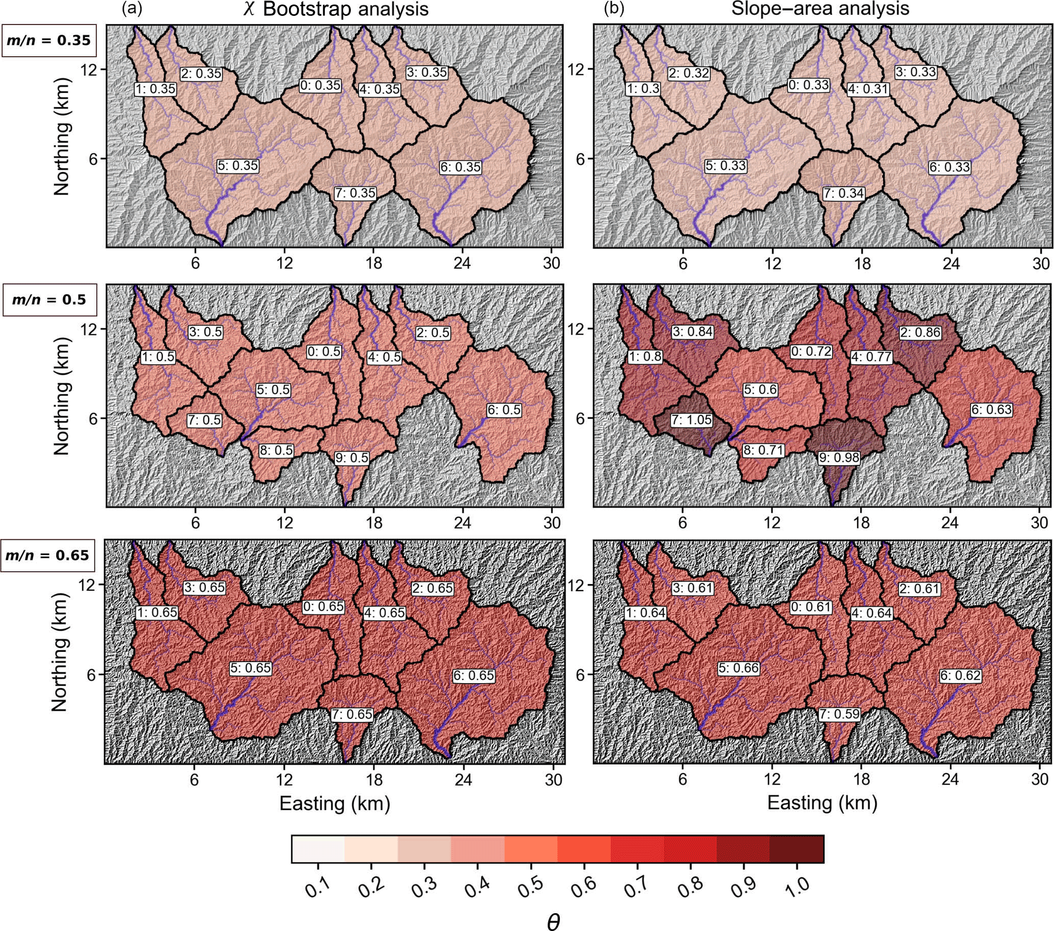
Figure 5Shaded relief plots of the model runs with temporally varying uplift, with drainage basins plotted by the best-fit θ predicted from the χ bootstrap analysis (column a), and slope–area analysis (column b). Each row represents a model run with a different m∕n ratio. The basins are coloured by the predicted θ, where darker colours indicate a higher concavity index. The extracted channel network for each basin is shown in blue.
We initialised the model runs using a low relief surface that is created using the diamond–square algorithm (Fournier et al., 1982). We found this approach resulted in drainage networks that contained more topological complexity than those initiated from simple sloping or parabolic surfaces. Our aim was to test the ability of each method to extract the correct m∕n ratio without assuming that the landscapes were in steady state; therefore, each simulation was forced with varying uplift through time to ensure that the channel networks were transient.
Each model was run with a baseline uplift rate of 0.5 mm yr−1, which was increased by a factor of 4 for a period of 15 000 years, then decreased back to the baseline for another 15 000 years. For the runs with n=2, the cycles were set to 10 000 years, which was necessary to preserve evidence of transience, as knickpoints propagate more rapidly through the channel network as n increases. Relief is very sensitive to model parameters, and we found in numerical experiments that basin geometry was sensitive to relief, mirroring the results of Perron et al. (2008). We wanted modelled landscapes to have comparable relief and similar basin geometry across our simulations to ensure similar landscape configurations for different values of m, n, and m∕n. We therefore calculated the χ coordinate and solved Eq. (5) to find the K value for each modelled landscape that produced a relief of 200 m at the location with the greatest χ value given an uplift rate of 0.5 mm yr−1.
We analysed these model runs using each of the methods of estimating the best-fit m∕n outlined in Sect. 2.2. We extracted a channel network from each model domain using a contributing area threshold of 9×10⁵ m2. We performed a sensitivity analysis of the methods to this contributing area threshold (see the Supplement) and found that the estimated best-fit m∕n ratios were insensitive to the value of the threshold.
Drainage basins were selected by setting a minimum and maximum basin area, 9×10⁶ and 4.5×10⁷ m2, respectively; these values were chosen so extracted basins represented a good balance between the number of extracted basins and the number of tributaries in each basin. Nested basins were removed, as were basins that bordered the edge of the model domain. We exclude basins on the domain boundaries as the calculation of the χ coordinate for the integral profile analysis is dependent on drainage area, which may not be realistic at the edge of the domain. Elimination of basins on the edge of the DEM is essential for real landscapes, as a basin beheaded by raster clipping will have incorrect χ values, and we wanted to ensure both simulations and analyses on real basins used the same extraction algorithms. For each basin, we identified the best-fit concavity index predicted in five ways (as described in the methods section): (i) regression of all χ–elevation data; (ii) use of χ–elevation data processed by our method of sampling points with the bootstrap method; (iii) minimisation of the disorder metric from χ–elevation data using a similar technique to Hergarten et al. (2016); (iv) regression of all slope–area data; and (v) regressions through slope–area data for individual segments of the main stem. For all but the final method, the analyses use all tributaries in the basins.
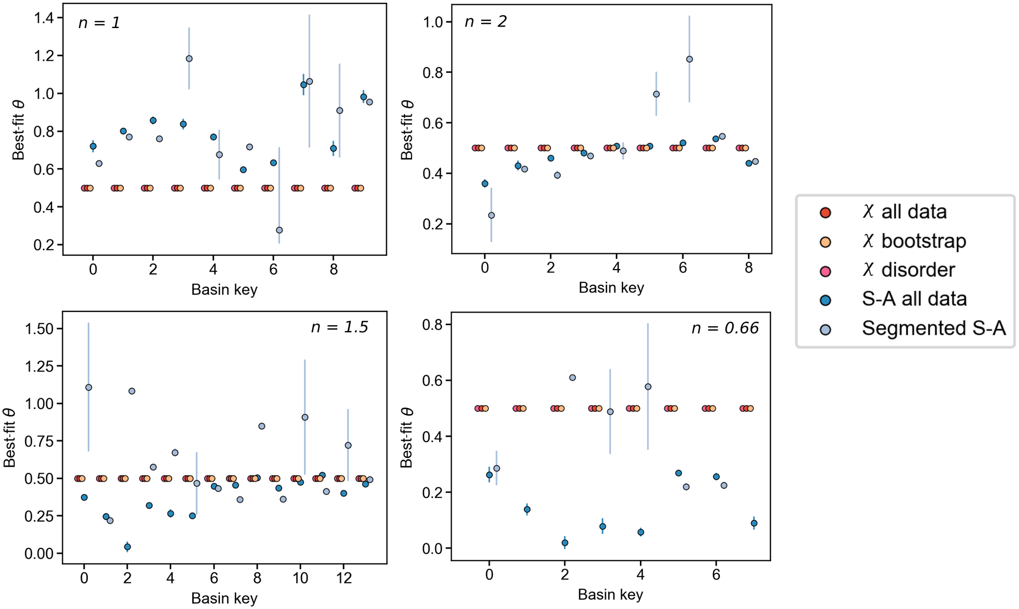
Figure 6Plots showing the predicted best-fit θ for each basin and each method for , where n = 1, n = 2, n = 1.5, and n = 0.66. The χ methods are shown in shades of red and the slope–area methods are shown in shades of blue.
Figure 5 shows the spatial distribution of the predicted m∕n ratio for a series of basins from these cyclic model runs, where m∕n = 0.35, 0.5, and 0.65, and n=1. We also plot the m∕n ratio predicted for each basin from all methods with varying values of n, an example of which is shown in Fig. 6. Our modelling results show that for each value of m∕n ratio tested, the method using all χ data identifies the correct ratio for every basin in the model domain. The bootstrap approach provides an estimate of the error on the best-fit m∕n ratio for each basin: Fig. 6 shows that there is no error on the predicted m∕n ratio, meaning that an identical m∕n ratio is predicted with each iteration of the bootstrap approach. The slope–area methods, in contrast, show more variation in the predicted m∕n ratio for each value of m∕n and n tested (Figs. 5 and 6). Furthermore, the segmented slope–area data show a higher uncertainty in the predicted m∕n ratio compared to the other methods. The results of the model runs for all values of m∕n and n are presented in the Supplement.
3.2 Spatially heterogeneous landscapes
Alongside these temporally transient scenarios, we also wished to test the ability of each method to identify the correct m∕n ratio in spatially heterogeneous landscapes, simulating the majority of real sites where lithology, climate, or uplift are generally non-uniform. Therefore, we performed additional runs where m∕n = 0.5, n=1, but U and K varied in space. We generated the model domains using the same diamond–square initial condition as the spatially homogeneous runs. For the run with spatially varying K, we calculate the steady-state value of K required to produce a surface with a relief of 400 m and an uplift rate of 1 mm yr−1 using the same method as for the previous runs. From this baseline value of K, we calculated a maximum K value which is 5 times that of the baseline. We then created 10 “patches” within the initial model domain where K was assigned randomly between the baseline and the maximum. These are rectangular in shape with K values that taper to the baseline K over 10 pixels. We acknowledge this pattern is not very realistic but emphasise that the aim is not to recreate real landscapes but rather to confuse the algorithms for quantifying the concavity index. This allows us to test if they can still detect modelled concavity indices even if we violate some of the assumptions implicit in our theoretical framework.
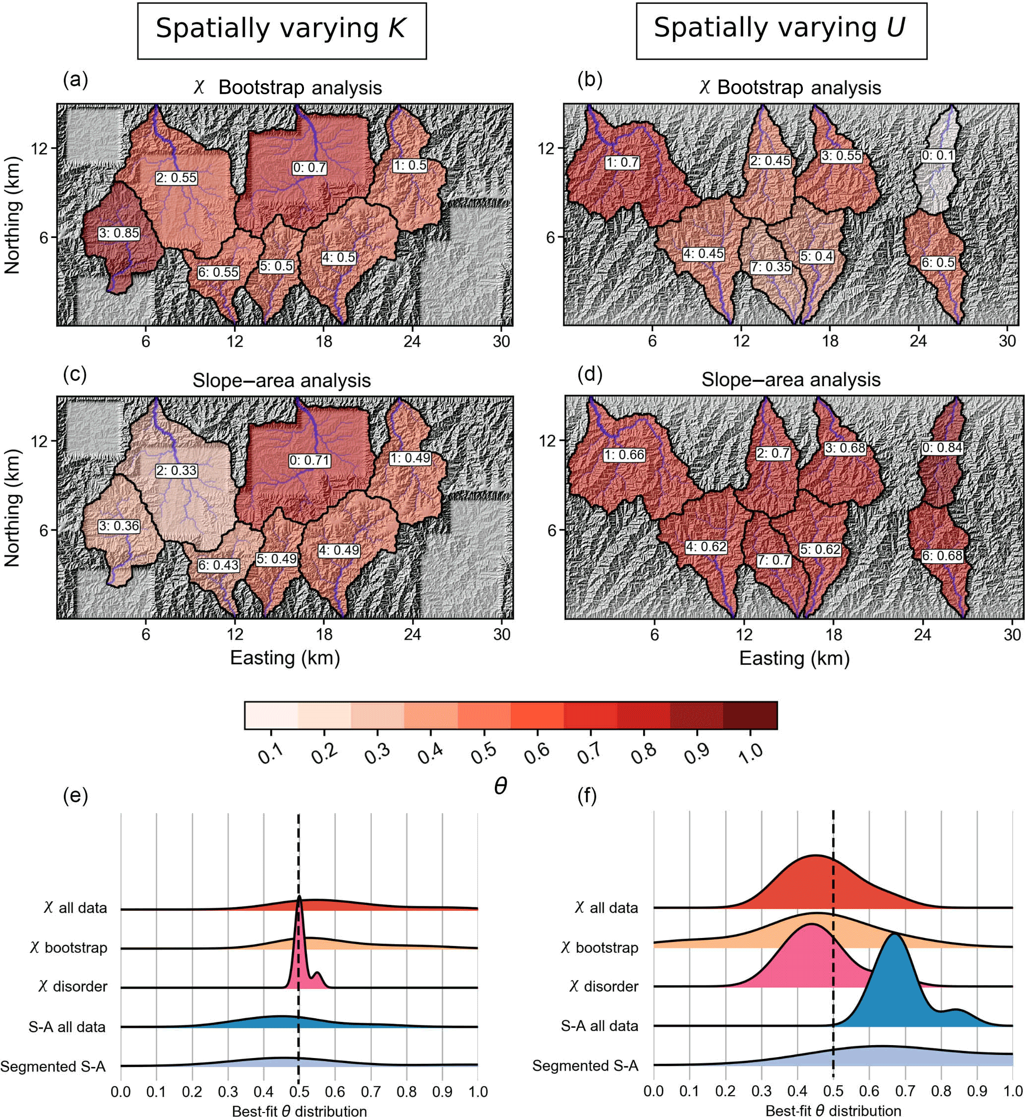
Figure 7Results of the model runs with spatially varying erodibility (K, a, c, e) and uplift (U, b, d, f). The rectangular patches of low relief are areas of high erodibility in (a), (c), and (e). Panels (a)–(d) show the spatial pattern of predicted θ from the χ bootstrap analysis and the slope–area analysis, where the basins are coloured by θ (darker colours indicate higher concavity index). Panels (e) and (f) show density plots of the distribution of θ for each method, where the dashed line marks the correct θ = 0.5.
For the spatially varying uplift run, we varied uplift in the N–S direction by modelling it as a half sine wave:
where y is the northing coordinate and L is the total length of the model domain in the y direction, UA is an uplift amplitude, set to 0.2 mm yr−1, and Umin is a minimum uplift, expressed at the north and south boundaries, of 0.2 mm yr−1. Both scenarios, with spatially varying erodibility and uplift, were run to approximately steady state; the maximum elevation change between 15 000-year printing intervals was less than a millimetre.
Inherent in each collinearity-based method of quantifying the most likely m∕n ratio is the assumption that U and K do not vary in space (Perron and Royden, 2013); our spatially heterogeneous experiments therefore violate basic assumptions of the integral method. These conditions, however, are likely true in virtually all natural landscapes. Therefore, our aim here was to test if we could recover m∕n ratios from numerical landscapes that are more similar to real landscapes than those with spatially homogeneous U and K.
Figure 7 shows the distribution of predicted m∕n ratios for the runs with spatially varying K and U from both the integral bootstrap approach and the slope–area method. In comparison to our model runs where K and U were uniform, each method performs worse at identifying the correct m∕n ratio of 0.5. However, in both model runs, the integral methods identified the correct ratio in a higher proportion of the drainage basins than the slope–area methods. Furthermore, the distribution of m∕n predicted by the integral methods reaches a peak at the correct m∕n ratios of 0.5, suggesting that even in spatially heterogeneous landscapes the methods can still be applied. Our run with the random distribution of erodibility patches shows that the correct calculation of the m∕n ratio is highly dependent on the spatial continuity of K; in basins contained within a single patch (e.g. basins 4, 5, and 6), the integral profile method correctly identified the m∕n ratios. Figure 8 shows example χ–elevation plots at varying m∕n ratios for basin 2, which encompasses several patches with varying K values. Within this basin, tributaries that drain a patch with the same K value are still collinear in χ–elevation space. Based on these results, we suggest that, in real landscapes, monolithologic catchments should be analysed wherever possible in order to select an appropriate concavity index.
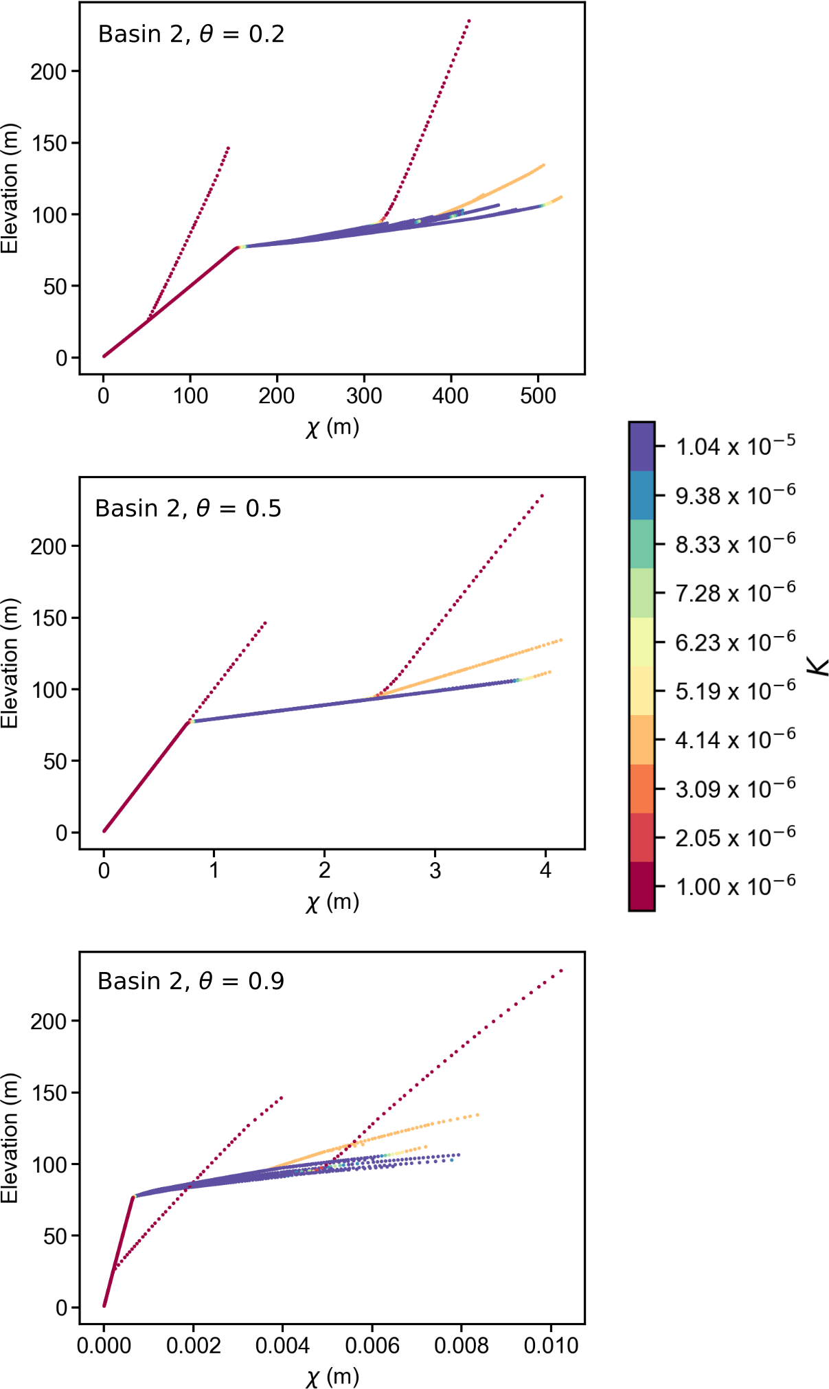
Figure 8Example χ–elevation plots for the model run with spatially varying erodibility, where points are coloured by K. The m∕n increases in each plot from 0.2 to 0.9. Tributaries with the same K value are collinear in χ–elevation space.
Our numerical modelling results suggest that the integral profile analysis is most successful in identifying the correct concavity index out of the entire range of m∕n and n values tested. However, these modelling scenarios cannot capture the range of complex tectonic, lithologic, and climatic influences present in nature. Therefore, we repeat our analyses on a range of different landscapes with varying climates, relief structures, and lithologies, to provide some examples of the variation in the concavity index predicted using each method. For each field site, topographic data were obtained from OpenTopography, using the seamless DEM generated from NASA's Shuttle Radar Topography Mission (SRTM) at a grid resolution of 30 m. The Supplement contains metadata for each site so readers can extract the same topographic data used here.
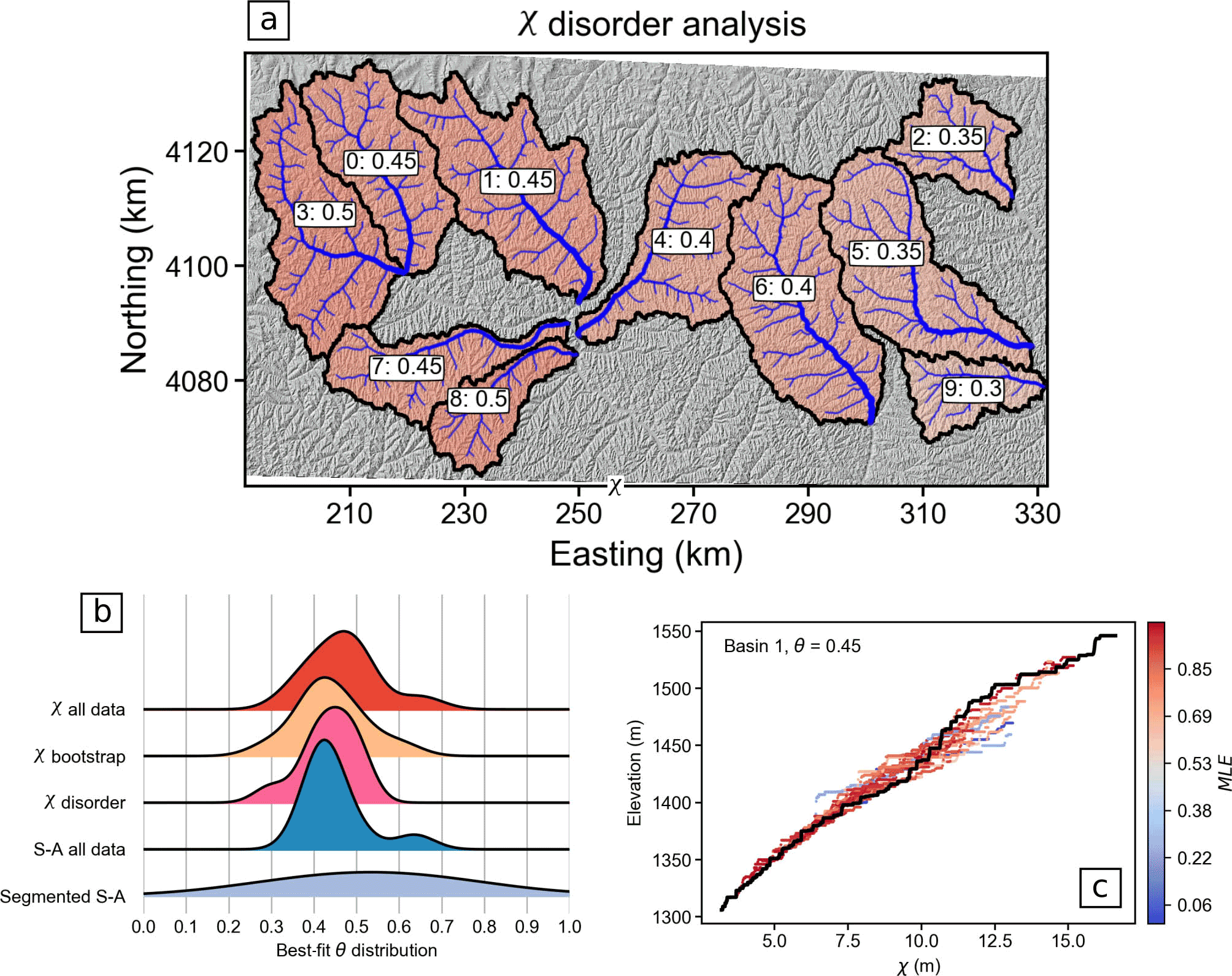
Figure 9Exploration of the most likely concavity indices in the Loess Plateau, China, Universal Transverse Mercator (UTM) zone 49 N. Basins with the most likely concavity index determined by the disorder method are displayed in panel (a); the basin number is followed by the most likely concavity index in the basin labels. The probability density of best-fit concavity index for all the basins (i.e. not the uncertainty within individual basins but rather the probability distribution of the best-fit concavity indices of all the basins) is displayed in panel (b). In basin 1, the most likely concavity index determined by the bootstrap and disorder methods is 0.45 and the χ–elevation plot for this concavity index is shown in panel (c).
4.1 An example of a relatively uniform landscape: Loess Plateau, China
In order to demonstrate the ability of the methods to constrain concavity indices in a relatively homogeneous landscape, we first analyse the Loess Plateau in northern China. The channels of the Loess Plateau are incising into wind-blown sediments that drape an extensive area of over 400 000 km2 (Zhang, 1980) and can exceed 300 m thickness (Fu et al., 2017). The plateau is underlain by the Ordos Block, a succession of non-marine Mesozoic sediments which has undergone stable uplift since the Miocene (B. Wang et al., 2017; Yueqiao et al., 2003). Although there have been both recent (Wang et al., 2016) and historic (Wang et al., 2006) changes in sediment discharge from the plateau, the friable substrate means that channel networks and channel profiles might be expected to adjust quickly to perturbations in erosion rate. Indeed, Willett et al. (2014) suggested, based on differences in the χ coordinate across drainage divides, that the channel networks in large portions of the plateau are geomorphically stable. The stable tectonic setting and homogeneous, weak substrate of the Loess Plateau make an ideal natural laboratory for testing our methods on relatively homogeneous channel profiles.
We ran each of the methods on an area of the Loess Plateau approximately 11 000 km2 in size near Yan'an, in the Chinese Shaanxi province (Fig. 9a). We find relatively good agreement between both the χ and slope–area methods of estimating the most likely concavity index. Figure 9b shows the probability distribution of concavities determined from the population of the most likely concavities from each basin (i.e. it does not include underlying uncertainty in each basin), but the peaks of these curves lie at a θ≈0.45 using both the disorder method and the bootstrap method, 0.4 using all slope–area data, and at approximately 0.5 using the all χ data method. This level of agreement gives the worker some confidence that channel steepness analyses in this area of the Loess Plateau using reference concavities between 0.4 and 0.5 should give an accurate representation of the relative steepness of the channels.
As well as determining the best-fit concavity index for the landscape as a whole, we can also examine the channel networks in individual basins: Fig. 9c shows the χ–elevation profiles for an example basin. In this basin, the tributaries are well aligned with the trunk channel at the most likely θ of 0.45, both using all the χ data and with the bootstrap approach. In our explorations of different landscapes, the Loess Plateau is the landscape that most resembles the idealised landscapes that we find in our model simulations. The Loess Plateau is notable for the homogeneity of its substrate over a large area; most locations on Earth are not as homogeneous.
4.2 An example of lithologic variability: Waldport, Oregon, USA
Many studies analysing the steepness of channel profiles are focused in areas where external factors, such as lithology or tectonics, are not uniform. Here, we select an example of a landscape with two dominant lithologic types in a location along the Oregon coast near the town of Waldport, Oregon (Fig. 10). The Oregon Coast Range is dominated by the Tyee Formation, made up primarily of turbidites deposited during the Eocene (Heller et al., 1987). In addition to these sedimentary units, our selected landscape also contains the Yachats Basalt, which erupted mostly as sub-areal flows between 3 and 9 m in thickness during the late Eocene (Davis et al., 1995). Erosion rates inferred from 10Be concentrations in stream sediments are between 0.11 to 0.14 mm yr−1 (Bierman et al., 2001; Heimsath et al., 2001), similar to rock uplift rates of 0.05–0.35 mm yr−1 inferred from marine terraces (Kelsey et al., 1994). Short-term erosion rates derived from stream sediments fall into the range of 0.07 to 0.18 mm yr−1 (Wheatcroft and Sommerfield, 2005), leading a number of authors to suggest that the Coast Range is in topographic steady state, where uplift is balanced by erosion (Reneau and Dietrich, 1991). Thus, our site contains a clear lithologic contrast but has been selected to minimise spatial variations in uplift or erosion rates.
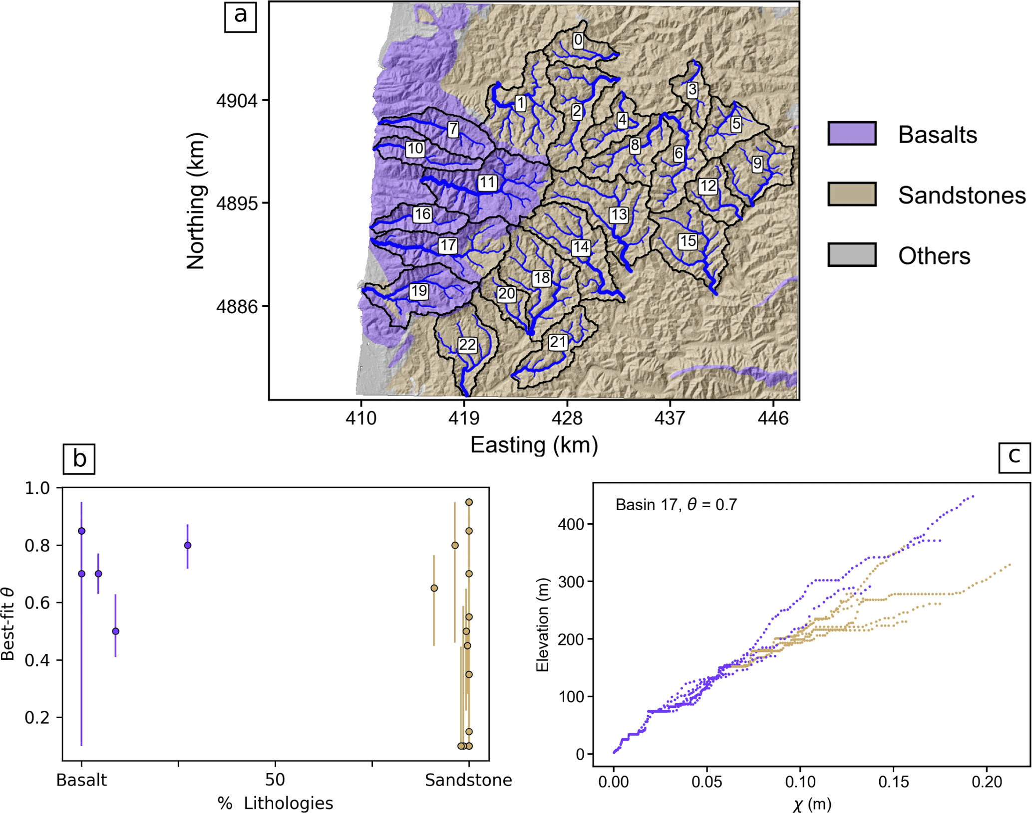
Figure 10Exploration of the most likely concavity index near Waldport, Oregon, UTM zone 10 N. Basin numbers and the underlying lithology is displayed in panel (a). The most likely concavity index determined by the bootstrap method as a function of the percent of each basin in the different lithologies is shown in panel (b). Panel (c) shows the χ–elevation plot for a basin that has two bedrock types; the channel pixels are coloured by lithology. The plot uses the typical concavity index for basalt (0.7).
We find that whereas basins developed on basalt have a relatively uniform concavity index of approximately 0.7, the most likely concavity indices in the sandstone show considerably more scatter (Fig. 10b), with a lower average θ. We present these data as an example of spatially varying concavity indices as a function of lithology. This is consistent with results of VanLaningham et al. (2006), who found high concavities in volcanic rocks around Waldport but lower elsewhere, and found high values of the concavity index in sedimentary rock but with a higher degree of scatter along the Oregon Coast Range.
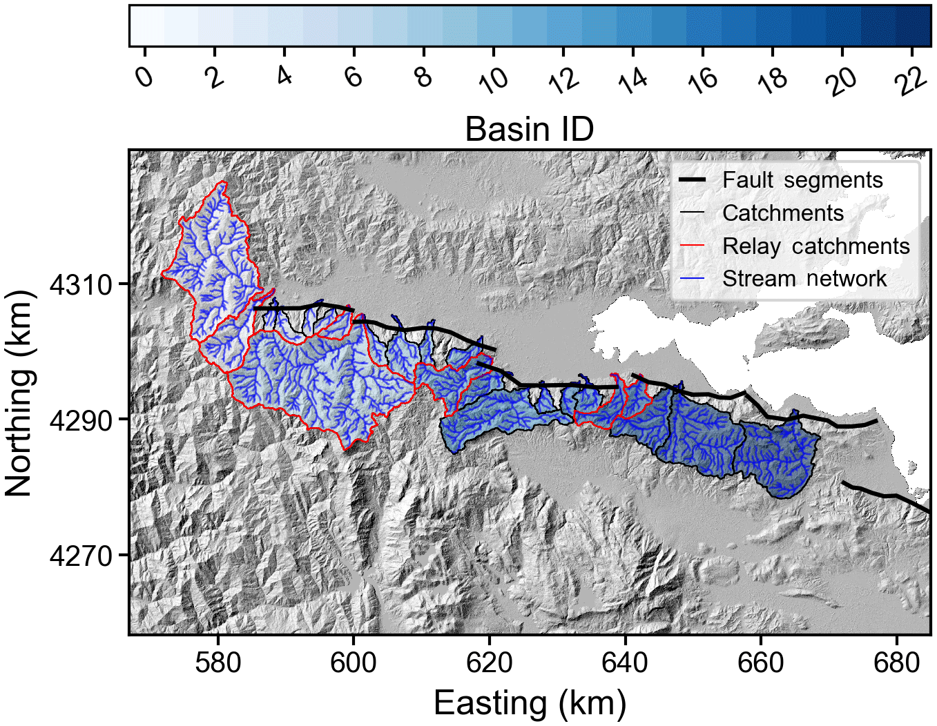
Figure 11Basins analysed near the Gulf of Evia, Greece, UTM zone 34 N, that interact with active normal faults previously studied by Whittaker and Walker (2015).
Whipple and Tucker (1999) suggested that the concavity index is controlled primarily by discharge–drainage area and channel width–drainage area relationships, which may be influenced by lithology, but other authors have found systematic variations in concavity indices with lithology (Duvall et al., 2004; Lima and Flores, 2017; VanLaningham et al., 2006). Lima and Flores (2017) suggested that the thickness of basalt flows could influence concavity indices, with different knickpoint propagation mechanisms in massive versus thinly bedded flows. Duvall et al. (2004) suggested that having hard rocks in headwaters and weak below might influence concavity indices, which may be tested by comparing concavity indices in both monolithologic basins and basins with mixed lithology. The χ profiles in basin 17 (Fig. 10c) are notable because this basin features two bedrock types: basalt in the lower reaches and sandstone in the headwaters. If the selected concavity index is too high, tributaries will fall below the trunk channel in χ–elevation space. In Fig. 10c, θ is chosen to reflect the typical value of the basalt basins, and tributary channels in the sandstone fall below the trunk channel, meaning that changes in the concavity index can be seen within basins. We therefore suggest that workers must be cautious when using a reference concavity index in determining channel steepness indices in basins with heterogeneous lithology.
4.3 An example of a tectonically active site: Gulf of Evia, Greece
The steepness of channel profiles and presence of steepened reaches (knickpoints) in tectonically active areas can reveal spatial patterns in the distribution of erosion and/or uplift (Densmore et al., 2007; DiBiase et al., 2010; Vanacker et al., 2015) and have the potential to allow identification of active faults (Kirby and Whipple, 2012). However, these systematic spatial patterns in channel steepness may challenge our ability to constrain the concavity index. Our third example is in a tectonically active landscape where we have found spatial variations in the most likely concavity index between catchments proximal to active normal faults. We explore a series of basins draining across faults in the Sperchios Basin, Gulf of Evia, Greece (Fig. 11), predominantly cut into clastic sediments (Eliet and Gawthorpe, 1995). Previous work (Whittaker and Walker, 2015) has demonstrated that catchment morphology reflects interaction with these faults. The rivers are typically characterised by convex longitudinal profiles that commonly have two knickpoints. The upper set of knickpoints is attributed to the initiation of faulting and the resulting growth of topography. The lower set of knickpoints is interpreted as the result of subsequent increase (3–5 ×) in throw rate due to fault linkage (Whittaker and Walker, 2015). The elevations of each group of knickpoints both scale with footwall relief, suggesting that fault throw rates scale with fault segment length. The Gulf of Evia therefore represents a natural experiment where uplift and erosion rates are expected to vary both temporally and spatially.
Steep, smaller catchments tend to drain across the footwalls of these faults, whilst larger catchments drain the landscape behind the faults, through the relay zones between fault segments. We derived the best-fit concavity index for each catchment following each of the five methods (Fig. 12). Given the presence of knickpoints along the river profiles, it is not appropriate to derive the concavity index by linear regression of all log[S]–log[A] data. We find that the concavity index estimated from segmented slope–area analysis is highly variable between catchments (Fig. 12, inset), with a tendency toward abnormally large values, exceeding the upper range of values typically predicted by incision models (Whipple and Tucker, 1999). Values of θ derived using the χ methods are predicted to be relatively low, typically 0.1–0.6 (Fig. 12), and whilst the χ methods do not agree perfectly, they do covary, and are for the most part within uncertainty of each other (with the exception of basins 1 and 20).
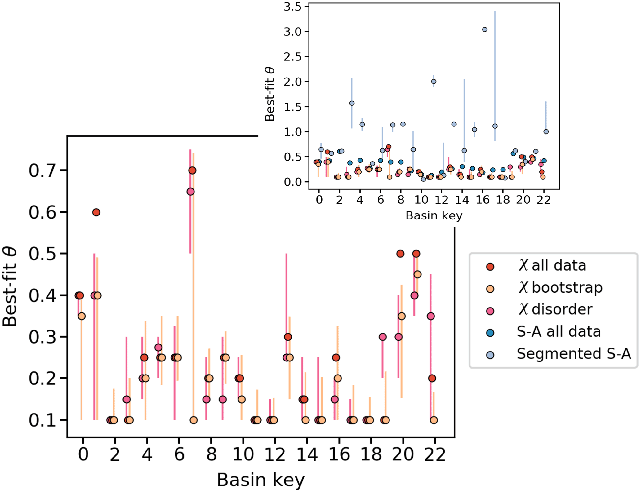
Figure 12The predicted best-fit θ determined using the χ methods (red points) and slope–area methods (blue points shown in inset). Basin numbers correspond to those plotted in Fig. 11.
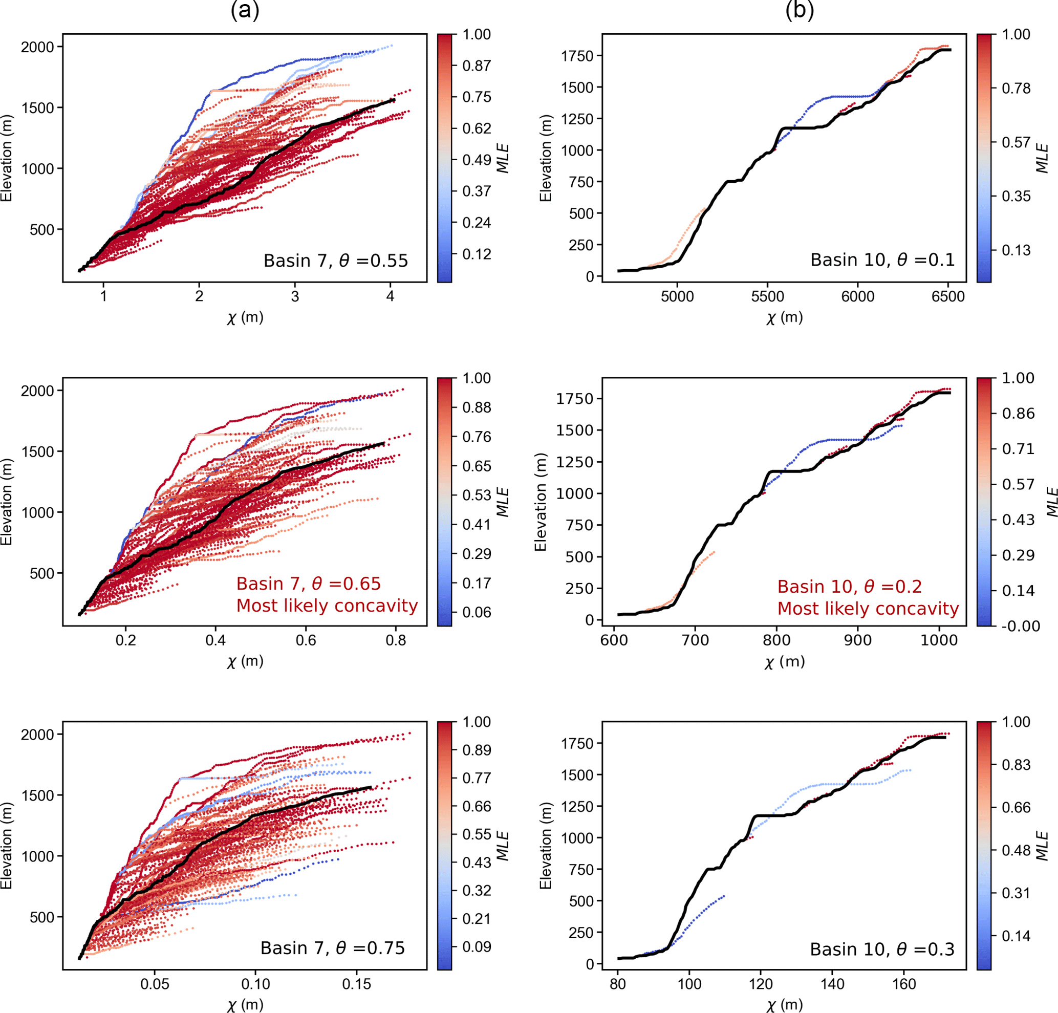
Figure 13Profile χ–elevation plots associated with best-fit θ for basin 7, a large catchment with many tributaries draining across a relay zone between normal fault segments (column a), and basin 10, a small, steep catchment draining directly across the footwall segment of a normal fault with few tributaries (column b). Note that MLE values depend on both the number of nodes and the vertical offset from the trunk channel.
A number of authors have suggested that in both highly transient and rapidly eroding landscapes processes other than fluvial plucking or abrasion become important in shaping the channel profile, such as debris flows and plunge pool erosion (DiBiase et al., 2015; Haviv et al., 2010; Scheingross and Lamb, 2017; Stock and Dietrich, 2003). Recent work has suggested that retreat of vertical waterfalls may result in similar concavities to fluvial incision processes operating in lower gradient settings (Shelef et al., 2018), whereas debris flows have been shown to lead to channels with low concavity indices (Stock and Dietrich, 2003). The lowest values of θ = 0.1 at the Evia site typically occur for the small, steep catchments draining across the footwalls of the fault segments (e.g. basin 10; Fig. 13), with higher θ values typical for catchments that do not cross faults or those that cross relay zones (e.g. basin 7; Fig. 13). Plots of χ–elevation such as in Fig. 13 demonstrate that there can be considerable variability in the morphology of tributaries as they respond to adjustment in the trunk channel.
Our aim here is not to provide a comprehensive examination of the topography and tectonic evolution of the Sperchios Basin (Whittaker and Walker, 2015) but to demonstrate the impact of tectonic transience on our ability to quantify the concavity index. Low concavity indices in steep, small catchments draining across the faults may reflect the contribution of debris flow processes to valley erosion at smaller drainage areas, which tends to lead to lower apparent concavity indices in the topography (Stock and Dietrich, 2003). Additionally, these catchments may in effect behave as fluvial hanging valleys (Wobus et al., 2006b). Concavity indices derived using the bootstrap points method are in all cases equal to or lower than values derived using all χ data. This is noteworthy because of the difference in how tributaries are weighted between the two techniques. Using all χ data, longer tributaries have more influence on the calculation of the most likely concavity index, whereas the bootstrap points method weights each tributary equally (since the same number of points are sampled on each tributary). Thus, if the steepness of the channels at low drainage area is influenced by debris flow processes (Stock and Dietrich, 2003), we would expect this to be more influential on the derived concavity index when using the bootstrap points method, resulting in lower θ values.
Finally, it is recognised that transient landscapes are likely settings for drainage network reorganisation (Willett et al., 2014). In the absence of lithologic variability, climate gradients and tectonic transience, gradients in χ in the channel network between adjacent drainage basins are predicted to indicate locations where drainage divides are migrating (toward the catchment with higher χ) and drainage network reorganisation is ongoing (Willett et al., 2014). On the other hand, numerical simulations suggest that spatial variability in uplift is more important than temporal gradients in uplift rates (Whipple et al., 2016). Rivers draining across normal fault systems are often routed through the relay zones between fault tips, where uplift rates are lowest, capturing and rerouting much of the drainage area above the footwall (Paton, 1992). In the Sperchios Basin, this has resulted in strong gradients in χ across topographic divides (Fig. 14), particularly between the large catchments draining the landscape behind the footwall (which have likely been gaining drainage area), and the short, steep catchments draining across the footwall (which have likely been truncated).

Figure 14Spatial distribution of the χ coordinate in the channel network calculated using A0 = 1 m2; θ = 0.45. Gradients in χ across topographic divides (black) can indicate planform disequilibrium such that the drainage network may be reorganising. Divides will tend to migrate from low values of χ towards high values in the channel network.
Our analysis of the topography in the Sperchios Basin, whilst not exhaustive, highlights that river profiles and the resulting concavities (and/or ksn) derived from topography are not alone sufficient to interpret the history of landscape evolution but must be considered alongside other observational data and in the context of a process-based understanding of landscape evolution and tectonics.
For over a century, geomorphologists have sought to link the steepness of bedrock channels to erosion rates, but any attempt to do so requires some form of normalisation. This normalisation is required because in addition to topographic gradient, the relative efficacy of incision processes is thought to correlate with other landscape properties that are a function of drainage area, such as discharge or sediment flux. Theory developed over the last four decades suggest that the concavity index may be used to normalise channel gradient, and over the last two decades many authors have compared the steepness of channels normalised to a reference concavity index derived from slope–area data (Kirby and Whipple, 2001; Snyder et al., 2000). In recent years, an integral method of channel analysis has also been developed (Perron and Royden, 2013) that can complement slope–area analysis and via alignment of tributaries provide an independent test of the concavity index.
In this contribution, we have developed a suite of methods to quantify the most likely concavity index using both slope–area analysis and the integral method. In addition to traditional slope–area methods, we also present methods of analysing χ-transformed channel networks that do not require the profiles to be linear from source to outlet but constrain concavity-based collinearity of each tributary and the trunk channel. In a second method, we quantify uncertainty on the predicted value of θ using a subset of points on the tributary network that are randomly assigned within a bootstrap sampling framework. We also test a similar disorder metric that is a minimum when tributaries and trunk channel are most collinear. We test these methods against idealised, modelled landscapes that obey the stream power incision model but have been subject to transient uplift, as well as spatially varying uplift and erodibility, where the concavity index is imposed through the ratio of the exponents m and n.
We find that χ-based methods are best able to reproduce the concavity indices imposed on the model runs. We recommend users calculate the most likely concavity indices using the bootstrap and disorder methods as these provide estimates of uncertainty, although the disorder method is the most tightly constrained of the χ-based methods. The most likely concavities determined from χ-based methods on transient landscapes have low uncertainty because the transient models do not violate any assumptions underlying χ-based methods. The spatially variable model runs, where assumptions of the χ method are violated, still perform better than slope–area analysis in extracting the correct concavity index. This gives us some confidence that in real landscapes, where non-uniform uplift and spatially varying erodibility are likely pervasive, calculated concavities may still reveal useful information about the incision processes. Thus, we hope future workers can calculate reliable, reproducible concavity indices for many small basins in regions with spatially varying uplift, climate, or lithology to test if patterns in the concavity index can be linked to variations in these landscape properties.
Code used for analysis is located at https://doi.org/10.5281/zenodo.1291889 (Mudd et al., 2018) and https://doi.org/10.5281/zenodo.1291889 (Mudd et al., 2017). Scripts for visualising the results can be found at https://github.com/LSDtopotools/LSDMappingTools (last access: 18 June 2018). We have also provided documentation detailing how to install and run the software, which can be found at https://lsdtopotools.github.io/LSDTT_documentation (last access: 18 June 2018). As part of the Supplement, we have also provided 45 example parameter files which can be used to reproduce the results of all analyses performed in this study. All topographic data used in this contribution are available through http://Opentopography.org (last access: 22 November 2017; NSF OpenTopography Facility, 2013).
The supplement related to this article is available online at: https://doi.org/10.5194/esurf-6-505-2018-supplement.
SMM and FJC wrote the code for the analysis, performed the numerical modelling and wrote the visualisation software. SMM, FJC, BG, and MDH performed the analysis on the real landscapes. SMM wrote the paper with contributions from other authors.
The authors declare that they have no conflict of interest.
We thank Rahul Devrani, Jiun Yee Yen, Ben Melosh, Julien Babault,
Calum Bradbury, and Daniel Peifer for beta testing the software. Reviews by
Liran Goren and Roman DiBiase substantially improved the
paper. This work was supported by Natural Environment Research Council grants
NE/J009970/1 to Simon M. Mudd and NE/P012922/1 to Fiona J. Clubb.
Boris Gailleton was funded by European Union Initial Training grant 674899 –
SUBITOP. All topographic data used for this study were SRTM 30 m data
obtained from http://Opentopography.org (last access: 22 November 2017;
NSF OpenTopography Facility, 2013).
Edited by: Jens
Turowski
Reviewed by: Roman DiBiase and Liran Goren
Aiken, S. J. and Brierley, G. J.: Analysis of longitudinal profiles along the eastern margin of the Qinghai-Tibetan Plateau, J. Mt. Sci., 10, 643–657, https://doi.org/10.1007/s11629-013-2814-2, 2013. a
Akaike, H.: A new look at the statistical model identification, IEEE T. Automat. Contr., 19, 716–723, https://doi.org/10.1109/tac.1974.1100705, 1974. a
Bierman, P., Clapp, E., Nichols, K., Gillespie, A., and Caffee, M. W.: Using Cosmogenic Nuclide Measurements In Sediments To Understand Background Rates Of Erosion And Sediment Transport, in: Landscape Erosion and Evolution Modeling, 89–115, Springer, Boston, MA, https://doi.org/10.1007/978-1-4615-0575-4_5, 2001. a
Braun, J. and Willett, S. D.: A very efficient O(n), implicit and parallel method to solve the stream power equation governing fluvial incision and landscape evolution, Geomorphology, 180–181, 170–179, https://doi.org/10.1016/j.geomorph.2012.10.008, 2013. a, b
Burbank, D. W., Leland, J., Fielding, E., Anderson, R. S., Brozovic, N., Reid, M. R., and Duncan, C.: Bedrock incision, rock uplift and threshold hillslopes in the northwestern Himalayas, Nature, 379, 505–510, https://doi.org/10.1038/379505a0, 1996. a
Clubb, F. J., Mudd, S. M., Attal, M., Milodowski, D. T., and Grieve, S. W.: The relationship between drainage density, erosion rate, and hilltop curvature: Implications for sediment transport processes, J. Geophys. Res.-Earth, 121, 1724–1745, https://doi.org/10.1002/2015JF003747, 2016. a
Conway, S. J., Balme, M. R., Kreslavsky, M. A., Murray, J. B., and Towner, M. C.: The comparison of topographic long profiles of gullies on Earth to gullies on Mars: A signal of water on Mars, Icarus, 253, 189–204, https://doi.org/10.1016/j.icarus.2015.03.009, 2015. a
Crosby, B. T., Whipple, K. X., Gasparini, N. M., and Wobus, C. W.: Formation of fluvial hanging valleys: Theory and simulation, J. Geophys. Res.-Earth, 112, F03S10, https://doi.org/10.1029/2006JF000566, 2007. a
Cyr, A. J., Granger, D. E., Olivetti, V., and Molin, P.: Quantifying rock uplift rates using channel steepness and cosmogenic nuclide-determined erosion rates: Examples from northern and southern Italy, Lithosphere, 2, 188–198, https://doi.org/10.1130/L96.1, 2010. a, b
Davis, A. S., Snavely, P., Gray, L.-B., and Minasian, D.: Petrology of Late Eocene lavas erupted in the forearc of central Oregon, U.S. Geological Survey Open-File Report, U.S. Dept. of the Interior, U.S. Geological Survey, Menlo Park, Calif, 1995. a
Demoulin, A.: Testing the tectonic significance of some parameters of longitudinal river profiles: the case of the Ardenne (Belgium, NW Europe), Geomorphology, 24, 189–208, https://doi.org/10.1016/S0169-555X(98)00016-6, 1998. a
Densmore, A. L., Gupta, S., Allen, P. A., and Dawers, N. H.: Transient landscapes at fault tips, J. Geophys. Res.-Earth, 112, F03S08, https://doi.org/10.1029/2006JF000560, 2007. a
DiBiase, R. A., Whipple, K. X., Heimsath, A. M., and Ouimet, W. B.: Landscape form and millennial erosion rates in the San Gabriel Mountains, CA, Earth Planet. Sc. Lett., 289, 134–144, https://doi.org/10.1016/j.epsl.2009.10.036, 2010. a, b, c
DiBiase, R. A., Whipple, K. X., Lamb, M. P., and Heimsath, A. M.: The role of waterfalls and knickzones in controlling the style and pace of landscape adjustment in the western San Gabriel Mountains, California, GSA Bulletin, 127, 539–559, https://doi.org/10.1130/B31113.1, 2015. a
Duvall, A., Kirby, E., and Burbank, D.: Tectonic and lithologic controls on bedrock channel profiles and processes in coastal California, J. Geophys. Res.-Earth, 109, F03002, https://doi.org/10.1029/2003JF000086, 2004. a, b
Eliet, P. P. and Gawthorpe, R. L.: Drainage development and sediment supply within rifts, examples from the Sperchios basin, central Greece, J. Geol. Soc., 152, 883–893, https://doi.org/10.1144/gsjgs.152.5.0883, 1995. a
Flint, J. J.: Stream gradient as a function of order, magnitude, and discharge, Water Resour. Res., 10, 969–973, https://doi.org/10.1029/WR010i005p00969, 1974. a, b, c
Fournier, A., Fussell, D., and Carpenter, L.: Computer Rendering of Stochastic Models, Commun. ACM, 25, 371–384, https://doi.org/10.1145/358523.358553, 1982. a
Fox, M., Goren, L., May, D. A., and Willett, S. D.: Inversion of fluvial channels for paleorock uplift rates in Taiwan, J. Geophys. Res.-Earth, 119, 1853–1875, https://doi.org/10.1002/2014JF003196, 2014. a
Fu, B., Wang, S., Liu, Y., Liu, J., Liang, W., and Miao, C.: Hydrogeomorphic Ecosystem Responses to Natural and Anthropogenic Changes in the Loess Plateau of China, Annu. Rev. Earth Planet. Sc., 45, 223–243, https://doi.org/10.1146/annurev-earth-063016-020552, 2017. a
Gasparini, N. M. and Brandon, M. T.: A generalized power law approximation for fluvial incision of bedrock channels, J. Geophys. Res.-Earth, 116, F02020, https://doi.org/10.1029/2009JF001655, 2011. a
Gasparini, N. M. and Whipple, K. X.: Diagnosing climatic and tectonic controls on topography: Eastern flank of the northern Bolivian Andes, Lithosphere, 6, 230–250, https://doi.org/10.1130/L322.1, 2014. a
Gilbert, G.: Geology of the Henry Mountains, USGS Unnumbered Series, Government Printing Office, Washington, D.C., 1877. a, b
Goren, L., Fox, M., and Willett, S. D.: Tectonics from fluvial topography using formal linear inversion: Theory and applications to the Inyo Mountains, California, J. Geophys. Res.-Earth, 119, 1651–1681, https://doi.org/10.1002/2014JF003079, 2014. a, b, c
Hack, J.: Studies of longitudinal profiles in Virginia and Maryland, U.S. Geological Survey Professional Paper 294-B, United States Government Printing Office, Washington, D.C., 1957. a
Hack, J.: Interpretation of erosional topography in humid temperate regions, Interpretation of Erosional Topography in Humid Temperate Regions, 258-A, 80–97, 1960. a
Harel, M. A., Mudd, S. M., and Attal, M.: Global analysis of the stream power law parameters based on worldwide 10Be denudation rates, Geomorphology, 268, 184–196, https://doi.org/10.1016/j.geomorph.2016.05.035, 2016. a, b, c
Harkins, N., Kirby, E., Heimsath, A., Robinson, R., and Reiser, U.: Transient fluvial incision in the headwaters of the Yellow River, northeastern Tibet, China, J. Geophys. Res.-Earth, 112, F03S04, https://doi.org/10.1029/2006JF000570, 2007. a
Haviv, I., Enzel, Y., Whipple, K. X., Zilberman, E., Matmon, A., Stone, J., and Fifield, K. L.: Evolution of vertical knickpoints (waterfalls) with resistant caprock: Insights from numerical modeling, J. Geophys. Res.-Earth, 115, F03028, https://doi.org/10.1029/2008JF001187, 2010. a
Heimsath, A. M., Dietrich, W. E., Nishiizumi, K., and Finkel, R. C.: Stochastic processes of soil production and transport: erosion rates, topographic variation and cosmogenic nuclides in the Oregon Coast Range, Earth Surf. Proc. Land., 26, 531–552, https://doi.org/10.1002/esp.209, 2001. a
Heller, P. L., Tabor, R. W., and Suczek, C. A.: Paleogeographic evolution of the United States Pacific Northwest during Paleogene time, Can. J. Earth Sci., 24, 1652–1667, https://doi.org/10.1139/e87-159, 1987. a
Hergarten, S., Robl, J., and Stüwe, K.: Tectonic geomorphology at small catchment sizes – extensions of the stream-power approach and the χ method, Earth Surf. Dynam., 4, 1–9, https://doi.org/10.5194/esurf-4-1-2016, 2016. a, b, c, d, e
Howard, A. D. and Kerby, G.: Channel changes in badlands, Geol. Soc. Am. Bull., 94, 739–752, https://doi.org/10.1130/0016-7606(1983)94<739:CCIB>2.0.CO;2, 1983. a
Hurst, M. D., Mudd, S. M., Attal, M., and Hilley, G.: Hillslopes Record the Growth and Decay of Landscapes, Science, 341, 868–871, https://doi.org/10.1126/science.1241791, 2013. a
Kelsey, H. M., Engebretson, D. C., Mitchell, C. E., and Ticknor, R. L.: Topographic form of the Coast Ranges of the Cascadia Margin in relation to coastal uplift rates and plate subduction, J. Geophys. Res.-Sol. Ea., 99, 12245–12255, https://doi.org/10.1029/93JB03236, 1994. a
Kirby, E. and Whipple, K.: Quantifying differential rock-uplift rates via stream profile analysis, Geology, 29, 415–418, https://doi.org/10.1130/0091-7613(2001)029<0415:QDRURV>2.0.CO;2, 2001. a, b, c
Kirby, E. and Whipple, K. X.: Expression of active tectonics in erosional landscapes, J. Struct. Geol., 44, 54–75, https://doi.org/10.1016/j.jsg.2012.07.009, 2012. a, b, c, d, e
Kirby, E., Whipple, K. X., Tang, W., and Chen, Z.: Distribution of active rock uplift along the eastern margin of the Tibetan Plateau: Inferences from bedrock channel longitudinal profiles, J. Geophys. Res.-Sol. Ea., 108, 2217, https://doi.org/10.1029/2001JB000861, 2003. a
Kobor, J. S. and Roering, J. J.: Systematic variation of bedrock channel gradients in the central Oregon Coast Range: implications for rock uplift and shallow landsliding, Geomorphology, 62, 239–256, https://doi.org/10.1016/j.geomorph.2004.02.013, 2004. a
Kwang, J. S. and Parker, G.: Landscape evolution models using the stream power incision model show unrealistic behavior when m∕n equals 0.5, Earth Surf. Dynam., 5, 807–820, https://doi.org/10.5194/esurf-5-807-2017, 2017. a
Lague, D.: The stream power river incision model: evidence, theory and beyond, Earth Surf. Proc. Land., 39, 38–61, https://doi.org/10.1002/esp.3462, 2014. a, b
Lague, D. and Davy, P.: Constraints on the long-term colluvial erosion law by analyzing slope-area relationships at various tectonic uplift rates in the Siwaliks Hills (Nepal), J. Geophys. Res.-Sol. Ea., 108, 2129, https://doi.org/10.1029/2002JB001893, 2003. a, b
Lima, A. G. and Flores, D. M.: River slopes on basalts: Slope-area trends and lithologic control, J. S. Am. Earth Sci., 76, 375–388, https://doi.org/10.1016/j.jsames.2017.03.014, 2017. a, b
Mandal, S. K., Lupker, M., Burg, J.-P., Valla, P. G., Haghipour, N., and Christl, M.: Spatial variability of 10Be-derived erosion rates across the southern Peninsular Indian escarpment: A key to landscape evolution across passive margins, Earth Planet. Sc. Lett., 425, 154–167, https://doi.org/10.1016/j.epsl.2015.05.050, 2015. a
Morisawa, M. E.: Quantitative Geomorphology of Some Watersheds in the Appalachian Plateau, Geol. Soc. Am. Bull., 73, 1025–1046, https://doi.org/10.1130/0016-7606(1962)73[1025:QGOSWI]2.0.CO;2, 1962. a
Mudd, S. M.: Detection of transience in eroding landscapes, Earth Surf. Proc. Land., 42, 24–41, https://doi.org/10.1002/esp.3923, 2016. a, b
Mudd, S. M., Attal, M., Milodowski, D. T., Grieve, S. W., and Valters, D. A.: A statistical framework to quantify spatial variation in channel gradients using the integral method of channel profile analysis, J. Geophys. Res.-Earth, 119, 138–152, https://doi.org/10.1002/2013JF002981, 2014. a, b, c, d, e
Mudd, S. M., Jenkinson, J., Valters, D, A., and Clubb, F. J.: MuddPILE the Parsimonious Integrated Landscape Evolution Model (Version v0.08), Zenodo, https://doi.org/10.5281/zenodo.997407, 2017. a, b
Mudd, S. M., Clubb, F. J., Gailleton, B., Hurst, M. D., Milodowski, D. T., and Valters, D. A.: The LSDTopoTools Chi Mapping Package (Version 1.11), Zenodo, https://doi.org/10.5281/zenodo.1291889, 2018. a
Niemann, J. D., Gasparini, N. M., Tucker, G. E., and Bras, R. L.: A quantitative evaluation of Playfair's law and its use in testing long-term stream erosion models, Earth Surf. Proc. Land., 26, 1317–1332, https://doi.org/10.1002/esp.272, 2001. a
NSF OpenTopography Facility: Shuttle Radar Topography Mission (SRTM) 90 m, NSF OpenTopography Facility, https://doi.org/10.5069/G9445JDF, 2013. a, b
Ouimet, W. B., Whipple, K. X., and Granger, D. E.: Beyond threshold hillslopes: Channel adjustment to base-level fall in tectonically active mountain ranges, Geology, 37, 579–582, https://doi.org/10.1130/G30013A.1, 2009. a
Paton, S.: Active normal faulting, drainage patterns and sedimentation in southwestern Turkey, J. Geol. Soc., 149, 1031–1044, https://doi.org/10.1144/gsjgs.149.6.1031, 1992. a
Perron, J. T. and Royden, L.: An integral approach to bedrock river profile analysis, Earth Surf. Proc. Land., 38, 570–576, https://doi.org/10.1002/esp.3302, 2013. a, b, c, d, e, f, g
Perron, J. T., Dietrich, W. E., and Kirchner, J. W.: Controls on the spacing of first-order valleys, J. Geophys. Res.-Earth, 113, F04016, https://doi.org/10.1029/2007JF000977, 2008. a
Playfair, J.: Illustrations of the Huttonian theory of the earth, Neill and Co. Printers, Edinburgh, 1802. a
Pritchard, D., Roberts, G. G., White, N. J., and Richardson, C. N.: Uplift histories from river profiles, Geophys. Res. Lett., 36, L24301, https://doi.org/10.1029/2009GL040928, 2009. a
Reneau, S. L. and Dietrich, W. E.: Erosion rates in the southern oregon coast range: Evidence for an equilibrium between hillslope erosion and sediment yield, Earth Surf. Proc. Land., 16, 307–322, https://doi.org/10.1002/esp.3290160405, 1991. a
Roberts, G. G. and White, N.: Estimating uplift rate histories from river profiles using African examples, J. Geophys. Res.-Sol. Ea., 115, B02406, https://doi.org/10.1029/2009JB006692, 2010. a
Roy, N. G. and Sinha, R.: Integrating channel form and processes in the Gangetic plains rivers: Implications for geomorphic diversity, Geomorphology, 302, 46–61, https://doi.org/10.1016/j.geomorph.2017.09.031, 2018. a
Royden, L. and Perron, J. T.: Solutions of the stream power equation and application to the evolution of river longitudinal profiles, J. Geophys. Res.-Earth, 118, 497–518, https://doi.org/10.1002/jgrf.20031, 2013. a, b, c
Royden, L., Clark, M., and Whipple, K. X.: Evolution of river elevation profiles by bedrock incision: analystical solutions for transient river profiles related to changing uplift and precipitation rates, in: EOS, Transactions of the American Geophysical Union, Vol. 81, Fall Meeting Supplement, 2000. a, b, c
Scheingross, J. S. and Lamb, M. P.: A Mechanistic Model of Waterfall Plunge Pool Erosion into Bedrock, J. Geophys. Res.-Earth, 122, 2079–2104, https://doi.org/10.1002/2017JF004195, 2017. a
Scherler, D., Bookhagen, B., and Strecker, M. R.: Tectonic control on 10Be-derived erosion rates in the Garhwal Himalaya, India, J. Geophys. Res.-Earth, 119, 83–105, https://doi.org/10.1002/2013JF002955, 2014. a
Schwanghart, W. and Scherler, D.: Bumps in river profiles: uncertainty assessment and smoothing using quantile regression techniques, Earth Surf. Dynam., 5, 821–839, https://doi.org/10.5194/esurf-5-821-2017, 2017. a
Seeber, L. and Gornitz, V.: River profiles along the Himalayan arc as indicators of active tectonics, Tectonophysics, 92, 335–367, https://doi.org/10.1016/0040-1951(83)90201-9, 1983. a
Shaler, N. S.: Spacing of rivers with reference to hypothesis of baseleveling, GSA Bulletin, 10, 263–276, https://doi.org/10.1130/GSAB-10-263, 1899. a
Shelef, E., Haviv, I., and Goren, L.: A potential link between waterfall recession rate and bedrock channel concavity, J. Geophys. Res.-Earth, https://doi.org/10.1002/2016JF004138, online first, 2018. a, b
Sklar, L. and Dietrich, W. E.: River Longitudinal Profiles and Bedrock Incision Models: Stream Power and the Influence of Sediment Supply, in: Rivers Over Rock: Fluvial Processes in Bedrock Channels, 237–260, American Geophysical Union, https://doi.org/10.1029/GM107p0237, 1998. a
Snyder, N. P., Whipple, K. X., Tucker, G. E., and Merritts, D. J.: Landscape response to tectonic forcing: Digital elevation model analysis of stream profiles in the Mendocino triple junction region, northern California, GSA Bulletin, 112, 1250–1263, https://doi.org/10.1130/0016-7606(2000)112<1250:LRTTFD>2.0.CO;2, 2000. a, b, c
Stock, J. and Dietrich, W. E.: Valley incision by debris flows: Evidence of a topographic signature, Water Resour. Res., 39, 1089, https://doi.org/10.1029/2001WR001057, 2003. a, b, c, d
Tarboton, D. G., Bras, R. L., and Rodriguez-Iturbe, I.: Scaling and elevation in river networks, Water Resour. Res., 25, 2037–2051, https://doi.org/10.1029/WR025i009p02037, 1989. a
Tucker, G. E. and Bras, R. L.: A stochastic approach to modeling the role of rainfall variability in drainage basin evolution, Water Resour. Res., 36, 1953–1964, https://doi.org/10.1029/2000WR900065, 2000. a
Vanacker, V., von Blanckenburg, F., Govers, G., Molina, A., Campforts, B., and Kubik, P. W.: Transient river response, captured by channel steepness and its concavity, Geomorphology, 228, 234–243, https://doi.org/10.1016/j.geomorph.2014.09.013, 2015. a, b
VanLaningham, S., Meigs, A., and Goldfinger, C.: The effects of rock uplift and rock resistance on river morphology in a subduction zone forearc, Oregon, USA, Earth Surf. Proc. Land., 31, 1257–1279, https://doi.org/10.1002/esp.1326, 2006. a, b
Wang, B., Kaakinen, A., and Clift, P. D.: Tectonic controls of the onset of aeolian deposits in Chinese Loess Plateau – a preliminary hypothesis, Int. Geol. Rev., 60, 945–955, https://doi.org/10.1080/00206814.2017.1362362, 2017. a
Wang, L., Shao, M., Wang, Q., and Gale, W. J.: Historical changes in the environment of the Chinese Loess Plateau, Environ. Sci. Policy, 9, 675–684, https://doi.org/10.1016/j.envsci.2006.08.003, 2006. a
Wang, S., Fu, B., Piao, S., Lü, Y., Ciais, P., Feng, X., and Wang, Y.: Reduced sediment transport in the Yellow River due to anthropogenic changes, Nat. Geosci., 9, 38–41, https://doi.org/10.1038/ngeo2602, 2016. a
Wang, Y., Zhang, H., Zheng, D., Yu, J., Pang, J., and Ma, Y.: Coupling slope–area analysis, integral approach and statistic tests to steady-state bedrock river profile analysis, Earth Surf. Dynam., 5, 145–160, https://doi.org/10.5194/esurf-5-145-2017, 2017. a, b
Wheatcroft, R. A. and Sommerfield, C. K.: River sediment flux and shelf sediment accumulation rates on the Pacific Northwest margin, Cont. Shelf Res., 25, 311–332, https://doi.org/10.1016/j.csr.2004.10.001, 2005. a
Whipple, K. X.: Bedrock Rivers and the Geomorphology of Active Orogens, Annu. Rev. Earth Planet. Sc., 32, 151–185, https://doi.org/10.1146/annurev.earth.32.101802.120356, 2004. a
Whipple, K. X. and Tucker, G. E.: Dynamics of the stream-power river incision model: Implications for height limits of mountain ranges, landscape response timescales, and research needs, J. Geophys. Res.-Sol. Ea., 104, 17661–17674, https://doi.org/10.1029/1999JB900120, 1999. a, b, c, d
Whipple, K. X., Forte, A. M., DiBiase, R. A., Gasparini, N. M., and Ouimet, W. B.: Timescales of landscape response to divide migration and drainage capture: Implications for the role of divide mobility in landscape evolution, J. Geophys. Res.-Earth, 122, 248–273, https://doi.org/10.1002/2016JF003973, 2016. a
Whipple, K. X., DiBiase, R. A., Ouimet, W. B., and Forte, A. M.: Preservation or piracy: Diagnosing low-relief, high-elevation surface formation mechanisms, Geology, 45, 91–94, https://doi.org/10.1130/G38490.1, 2017. a
Whittaker, A. C. and Walker, A. S.: Geomorphic constraints on fault throw rates and linkage times: Examples from the Northern Gulf of Evia, Greece, J. Geophys. Res.-Earth, 120, 137–158, https://doi.org/10.1002/2014JF003318, 2015. a, b, c, d
Willett, S. D., McCoy, S. W., Perron, J. T., Goren, L., and Chen, C.-Y.: Dynamic Reorganization of River Basins, Science, 343, 1248765, https://doi.org/10.1126/science.1248765, 2014. a, b, c
Wobus, C. W., Whipple, K. X., Kirby, E., Snyder, N., Johnson, J., Spyropolou, K., Crosby, B., and Sheehan, D.: Tectonics from topography: Procedures, promise, and pitfalls, Geol. S. Am. S., 398, 55–74, https://doi.org/10.1130/2006.2398(04), 2006a. a, b, c, d, e, f
Wobus, C. W., Crosby, B. T., and Whipple, K. X.: Hanging valleys in fluvial systems: Controls on occurrence and implications for landscape evolution, J. Geophys. Res.-Earth, 111, F02017, https://doi.org/10.1029/2005JF000406, 2006b. a, b, c, d, e
Yueqiao, Z., Yinsheng, M., Nong, Y., Wei, S., and Shuwen, D.: Cenozoic extensional stress evolution in North China, J. Geodynam., 36, 591–613, https://doi.org/10.1016/j.jog.2003.08.001, 2003. a
Zhang, Z.: Loess in China, GeoJournal, 4, 525–540, https://doi.org/10.1007/BF00214218, 1980. a