the Creative Commons Attribution 4.0 License.
the Creative Commons Attribution 4.0 License.
 | 29 Aug 2018
Assessing the large-scale impacts of environmental change using a coupled hydrology and soil erosion model
Joris P. C. Eekhout
Wilco Terink
Joris de Vente
Assessing the impacts of environmental change on soil erosion and sediment yield at the large catchment scale remains one of the main challenges in soil erosion modelling studies. Here, we present a process-based soil erosion model, based on the integration of the Morgan–Morgan–Finney erosion model in a daily based hydrological model. The model overcomes many of the limitations of previous large-scale soil erosion models, as it includes a more complete representation of crucial processes like surface runoff generation, dynamic vegetation development, and sediment deposition, and runs at the catchment scale with a daily time step. This makes the model especially suited for the evaluation of the impacts of environmental change on soil erosion and sediment yield at regional scales and over decadal periods. The model was successfully applied in a large catchment in southeastern Spain. We demonstrate the model's capacity to perform impact assessments of environmental change scenarios, specifically simulating the scenario impacts of intra- and inter-annual variations in climate, land management, and vegetation development on soil erosion and sediment yield.
- Article
(11032 KB) - Full-text XML
-
Supplement
(164 KB) - BibTeX
- EndNote


Climate change will likely affect soil erosion and sediment yield at a wide variety of scales (Burt et al., 2016; Li et al., 2006; Nearing et al., 2004). However, assessing the impacts of environmental change on soil erosion and sediment yield at the large catchment scale remains one of the main challenges in soil erosion modelling (Poesen, 2018; de Vente et al., 2013). Most soil erosion and sediment yield models adopt simplified model formulations, are applied at low temporal resolutions, and in many cases only partly represent the impacts of changes in land use or climate conditions. This often leads to unreliable results that do not sufficiently increase process understanding or support decision making (de Vente et al., 2013). To overcome part of these limitations, we present a process-based, large-scale, soil erosion model, coupled to a hydrological model, which accounts for the most relevant factors determining soil erosion by water, including saturated and infiltration excess surface runoff, dynamic vegetation development, and sediment deposition.
Essentially, soil erosion by water occurs due to the impact of raindrops, overland flow, and river flow. Therefore, it is crucial to quantify raindrop impact, overland flow, and possible interactions with vegetation cover. Soil erosion due to the impact of raindrops is a function of the amount and the size of the raindrops that reach the soil surface (Morgan, 2005). Vegetation cover can reduce the impact of raindrops by interception, separating the precipitation into direct throughfall, which has a high impact, and leaf drainage, which has a lower impact (Morgan and Nearing, 2011). Therefore, assessment of soil erosion needs to account for spatial and temporal changes in vegetation cover. Nevertheless, most large-scale soil erosion assessments do not consider dynamic seasonal and inter-annual vegetation development. Previous studies have also shown that cropping patterns, inter-annual precipitation variability, and land use changes can have a significant impact on soil erosion rates (Maetens et al., 2012).
Soil erosion is also a function of runoff (Morgan, 2005). Runoff generation depends on surface and subsurface processes and is a function of precipitation volume and intensity, soil moisture, and soil hydraulic properties (Kirkby, 1988). Process-based models often incorporate a separate hydrological model to simulate surface runoff generation, which then directly forces soil erosion by runoff (Morgan, 2005). Surface runoff may be generated by several distinct processes, of which saturation excess and infiltration excess are the most common (Beven, 2012). Saturation excess surface runoff occurs when the soil water content reaches saturation, while infiltration excess surface runoff occurs when the precipitation intensity exceeds the soils infiltration capacity. However, many large-scale soil erosion models only consider saturation excess surface runoff, disregarding the infiltration excess surface runoff mechanism. Infiltration excess surface runoff is a sub-daily process that is often only implemented in event-scale models (Morgan et al., 1998; Nearing et al., 1989). Infiltration excess surface runoff is an especially important process in areas where the major part of soil erosion takes place during extreme rainfall events with high precipitation intensities (Farnsworth and Milliman, 2003; González-Hidalgo et al., 2007, 2012; López-Bermúdez et al., 2002; Mulligan, 1998).
Assessing catchment sediment yield further requires the evaluation of the sediment transport capacity and sediment deposition. Sediment deposition occurs when the sediment transport capacity of the runoff is exceeded and basically depends on the interaction between the texture of the detached soil material, flow velocity, and the roughness of the surface (Rose et al., 1983). Large particles are more likely to be deposited close to the source, while small particles are more easily brought and maintained into transport. The roughness of the surface is a combination of the soil roughness and vegetation roughness (Chow, 1959). Many studies have highlighted the importance of accounting for sediment transport and sediment deposition, claiming that a large part of the eroded sediment is often deposited close to its source (Walling, 1983; de Vente et al., 2007). However, many large-scale soil erosion models insufficiently consider this process or only simulate soil detachment processes.
From the available soil erosion models, process-based models aim to incorporate the most relevant processes driving soil detachment, sediment transport, and deposition, as described in the previous paragraphs, see Morgan (2005) for an overview of process-based models. Process-based models are often run at small spatial (hillslope to small catchment) and temporal scales (sub-hourly to daily time steps). Most detailed assessments are obtained from event-scale model applications in process-based models, such as WEPP (Nearing et al., 1989) and EUROSEM (Morgan et al., 1998), which require detailed input data, such as (sub-)hourly precipitation and topographic data, and incorporate a large number of calibration parameters (Govers, 2011). While these models present a strong potential to provide increased process understanding, it is often infeasible to obtain all required input data for large catchments. Furthermore, the high uncertainty regarding how input data and model parameters will change under scenarios of environmental change severely limits their application in large-scale assessments.
At larger scales, soil erosion is often assessed using empirical erosion models, see de Vente et al. (2013) for an overview. These models are derived from field studies where soil erosion has been observed under different land use, management, soil, climate, and topographical conditions. The most well known and applied empirical model is the Universal Soil Loss Equation (Wischmeier and Smith, 1978) and its derivatives RULSE (Renard et al., 1997) and MUSLE (Williams, 1995). While the empirical formulations of the USLE were obtained at plot-scale, the model is often applied at much larger scales, sometimes in combination with a sediment transport capacity equation or a sediment delivery ratio to assess sediment yield (Van Rompaey et al., 2001; de Vente et al., 2008). Due to their simplicity, the USLE and its derivatives can be applied with a relatively limited amount of input data. However, their main restriction is the limited number of processes accounted for (e.g. the USLE and RUSLE based models only consider sheet and rill erosion) and the limited potential to evaluate the impacts of changes in climate and land management (Govers, 2011; de Vente et al., 2013). Furthermore, these models are typically applied at annual time steps, largely neglecting intra-annual variation of climate and vegetation conditions.
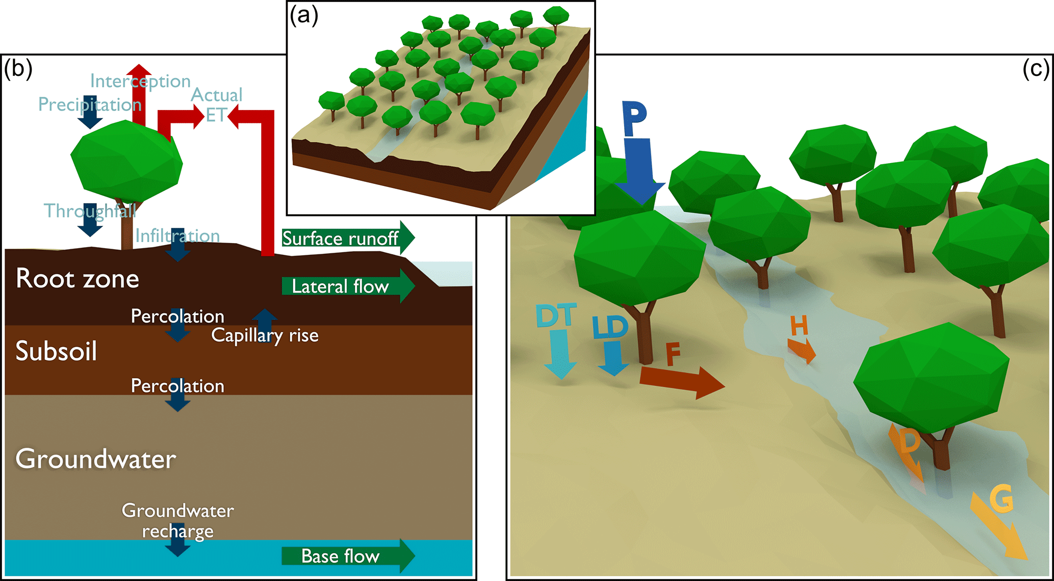
Figure 1Overview of the model: (a) representation of a single cell; (b) the hydrological processes, where ET is evapotranspiration; and (c) the soil erosion processes, where P is precipitation, DT is direct throughfall (Eq. 14), LD is leaf drainage (Eq. 13), F is detachment by raindrop impact (Eq. 18), H is detachment by runoff (Eq. 19), D is immediate deposition (Eq. 20), and G is sediment routed to downstream cells (Eq. 27).
Most current soil erosion models have a limited potential for application at larger temporal and spatial scales (i.e. process-based models) or lack sufficient representation of the underlying soil detachment and sediment transport processes and sensitivity to changes in land use or climate (i.e. empirical models), making them of limited use for scenario studies and process understanding. Here, we present a process-based soil erosion model based on the integration of the Morgan–Morgan–Finney erosion model (Morgan and Duzant, 2008) and the spatially distributed hydrological model “Spatial Processes in HYdrology” (Terink et al., 2015). This integrated model overcomes many of the limitations of previous large-scale soil erosion models, as it includes a more complete representation of crucial processes, such as surface runoff generation, dynamic vegetation development, and sediment deposition, and runs at the catchment scale with a daily time step. This makes the model especially suitable for the evaluation of the inter- and intra-annual impacts of environmental change on soil erosion and sediment yield at large spatial and temporal scales. In the next paragraphs we first present the different model components and enhancements as compared to previous models. We then illustrate its functionality and potential for scenario studies by applying the model to the upper Segura catchment in southeastern Spain under present and projected future climate conditions.
2.1 Model overview
The SPHY–MMF model presented here is an integration of the (Modified) Morgan–Morgan–Finney soil erosion model into the SPHY hydrological model (version 2.1). Figure 1 shows the main hydrological and soil erosion processes considered by the model. SPHY is a spatially distributed “leaky-bucket” type model that simulates hydrological processes on a cell-by-cell basis at a daily time step (Terink et al., 2015). The model is written in the Python programming language using the PCRaster dynamic modelling framework (Karssenberg et al., 2010). MMF is a conceptual soil erosion model that is originally applied with an annual time step. Here we present a modification of the model at a daily time step, fully integrated with the SPHY model. MMF receives input from the SPHY model, such as effective precipitation (throughfall), runoff, and canopy cover for calculation of erosion and deposition processes. The model parameters are presented in Table S1 in the Supplement. A video abstract (Eekhout and de Vente, 2018) is available that explains the most important aspects of the model.
2.2 Hydrological model
SPHY simulates most relevant hydrological processes (Fig. 1b), such as interception, evapotranspiration, dynamic evolution of vegetation cover, surface runoff, and lateral and vertical soil moisture flow at a daily time step. The model is described in full detail by Terink et al. (2015); therefore, here we only provide a summary of the processes that are simulated by the model, some hydrological processes that have been changed with respect to the original SPHY model, and a detailed description of the processes that are related to the integration of MMF.
SPHY requires daily precipitation and temperature maps as input. Effective precipitation is determined by subtracting canopy storage and interception from precipitation. Canopy storage is determined from the leaf area index (LAI), which is derived from normalized differenced vegetation index (NDVI) images. Reference evapotranspiration is determined using the Hargreaves equation (Hargreaves and Samani, 1985), which is subsequently multiplied by the crop coefficient to obtain the potential evapotranspiration. The crop coefficient is determined from the NDVI images using a linear relationship. Actual evapotranspiration is obtained by multiplying the potential evapotranspiration by a reduction factor for water deficit or water surplus, which are functions of current soil water content, soil hydraulic properties, and plant-specific water need. Surface runoff is determined by a daily implementation of the Green–Ampt formula (Heber Green and Ampt, 1911) and is a function of infiltration, effective precipitation, and soil hydraulic properties. The soil profile consists of three layers, i.e. root-zone, subzone, and groundwater layer. Water can percolate from the root-zone to the subzone and from the subzone to the groundwater layer. Water travels from the subzone to the root zone through capillary rise. Water drains from the root zone as lateral flow and from the groundwater layer as baseflow. The total runoff is the sum of surface runoff, lateral flow, and baseflow. All soil processes are functions of current water content (in the respective layers) and soil hydraulic properties, i.e. saturated hydraulic conductivity, saturated water content, field capacity, and wilting point. Water is routed using a single flow algorithm (Karssenberg et al., 2010). A flow recession coefficient accounts for flow delay from channel friction. When reservoirs are present, the user can opt to include an advanced routing scheme accounting for reservoir storage and outflow.
2.2.1 Evapotranspiration
The actual evapotranspiration (ETa) is determined by multiplying the potential evapotranspiration with the reduction parameters for water surplus and water deficit conditions. In the current version of the hydrological model we have changed the reduction parameter for water shortage conditions using the method proposed by Allen et al. (1998):
where Ks is the reduction parameter for water shortage (–), TAW is the total available water in the root zone (mm), Dr is the root-zone depletion (mm), and p is the depletion fraction (–). The total available water TAW is defined as
where θFC is the soil water content at field capacity (mm) and θWP is the soil water content at wilting point (mm). The root-zone depletion Dr is defined as
where θ is the current soil water content (mm). The depletion fraction p is defined as the fraction of TAW that a crop can extract from the root zone without suffering water stress, which is determined by the following equation:
where ptabular is a land use specific tabular value of the depletion fraction (–) and ETpot is the potential evapotranspiration (mm). Values for the land use specific tabular value of the depletion fraction can be obtained from Table 22 in Allen et al. (1998).
Open water evaporation is determined in the reservoir cells. In these cells all soil hydraulic processes are turned off and runoff equals precipitation minus open water evaporation. Reservoir cells cannot dry up, i.e. we assume that there is always water present in the reservoir cells. Open water evaporation is determined as follows:
where kcopen−water is the crop coefficient value for open water evaporation (–) and ETref is the reference evapotranspiration (mm). We set kcopen−water to a value of 1.2, following Allen et al. (1998). In each time step the open water evaporation is subtracted from the reservoir storage.
2.2.2 Infiltration excess surface runoff
The original SPHY model simulates saturated surface runoff but not infiltration excess surface runoff. Therefore, we have incorporated an infiltration excess equation at a daily time step, based on the Green–Ampt formula (Heber Green and Ampt, 1911). We assumed a constant infiltration rate (f) (mm), which is determined for each cell and each day by
where Keff is the effective hydraulic conductivity (mm), θsat is the saturated water content (mm), θ is the actual water content (mm), and λ is a calibration parameter (–). Bouwer (1969) suggested an approximation of Keff≈0.5 Ksat. We included a calibration parameter (k) in order to be able to change the value of Keff as a fraction of Ksat (Keff=kKsat).
Infiltration excess surface runoff occurs when the precipitation intensity exceeds the infiltration rate f (Beven, 2012). Analysis of hourly precipitation time series for 25 years (1991–2015) from 5 precipitation stations in a large catchment in southeastern Spain showed that, on average, the highest precipitation intensity was recorded in the first hour of a rain storm and decreased linearly until the end of the storm. We assumed a triangular-shaped precipitation intensity p(t) (mm hr−1) according to the following:
where α is the fraction of daily rainfall that occurs in the hour with the highest intensity (–), P is the daily rainfall (mm), and t is an hourly time step. Daily infiltration excess surface runoff Qsurf is determined as
2.2.3 Dynamic vegetation processes
SPHY–MMF contains a dynamic vegetation module that allows for the characterisation of the seasonal and inter-annual differences in vegetation cover and resulting canopy storage, interception, and precipitation throughfall. The latter is subsequently used in both the hydrological and soil erosion model. A time series of NDVI images is used as input for the dynamic vegetation module. NDVI images may only be available for a limited period, e.g. from 2000 to the present for MODIS NDVI images (Didan, 2015). Therefore, in Sect. 3 we present a method to obtain NDVI images for historical and future model assessments. The LAI is determined from the individual NDVI images using the following logarithmic relation, which is valid for vegetation that is evenly distributed over a surface (Sellers et al., 1996):
where LAImax is the maximum LAI (–), fPAR is the fraction of the photosynthetically active radiation (–), and fPARmax is the maximum fPAR (–), which is set to 0.95 (Sellers et al., 1996). The maximum LAI (LAImax) is vegetation dependent; values for several vegetation types can be found in Sellers et al. (1996). The fraction of the photosynthetically active radiation fPAR is determined as follows:
where SR is a transformation of NDVI (–), SRmin and SRmax are the minimum and maximum SR values (–), respectively, and fPARmin is the minimum fPAR (–), which is set to 0.001 (Sellers et al., 1996). fPAR is bounded by fPARmin and fPARmax. SR is determined as follows:
SRmin and SRmax are determined with Eq. (11), applying an NDVI value corresponding to the 5 % and 98 % quantiles, respectively.
2.3 Soil erosion simulation with a daily based Morgan–Morgan–Finney model
The soil erosion model is based on the Modified MMF model (Morgan and Duzant, 2008). In the current model (Fig. 1c), total soil erosion is calculated from detachment by raindrop impact and detachment by runoff, while sediment yield is calculated by routing detached sediment, considering within cell deposition and sediment transport capacity. Detachment of soil particles from raindrop impact is determined from the total rainfall energy, which is determined for direct throughfall and leaf drainage, respectively. Detachment of soil particles by runoff is determined from the accumulated runoff from the hydrological model. Both soil erosion equations account for the fraction of the soil covered by stones and vegetation or snow and are determined separately for three texture classes (sand, silt, and clay). Within cell deposition is calculated as a function of vegetation and surface roughness. The remainder of the detached sediment is taken into transport and routed through the catchment, taking the transport capacity of the flow and the trapping efficiency of the reservoirs into account. The next paragraphs provide a detailed description of all of these processes.
2.3.1 Estimation of rainfall energy
The total kinetic energy of the effective precipitation (KE, J m−2) is used to determine the detachment of soil particles by raindrop impact and is defined as
where KELD is the kinetic energy of the leaf drainage (J m−2) and KEDT is the kinetic energy of the direct throughfall (J m−2).
The kinetic energy of the leaf drainage is based on Brandt (1990):
where LD is the leaf drainage (mm) and PH is the plant height (m), specified for each land use class.
The kinetic energy of the direct throughfall is based on a relationship described by Marshall and Palmer (1948), which is representative of a wide range of environments (Morgan, 2005):
where DT is the direct throughfall (mm) and I is the intensity of the erosive precipitation (mm h−1). The intensity of the erosive precipitation is a model parameter and varies according to geographical location. Morgan and Duzant (2008) proposed 10 mm h−1 for temperate climates, 25 mm h−1 for tropical climates, and 30 mm h−1 for strongly seasonal climates (e.g. Mediterranean, tropical monsoon).
The leaf drainage (LD) (the precipitation that reaches the soil surface as flow or drips from the leaves and stems of the vegetation) and direct throughfall (DT) (the precipitation that reaches the soil surface directly through gaps in the vegetation cover), from Eqs. (13) and (14), are obtained from the effective precipitation, also known as throughfall (Peff, mm). The effective precipitation from the hydrological model is first corrected for the slope angle, following Choi et al. (2017):
where Peff is the effective precipitation (mm) and S is the slope (∘).
Leaf drainage is determined as
where CC is the canopy cover (proportion between zero and unity). The canopy cover is either introduced by a land use class specific tabular value or determined by the vegetation module. When the vegetation module is used, the canopy cover is obtained from the LAI (Eq. 9), maximised by 1.
Direct throughfall becomes
2.3.2 Detachment of soil particles
Detachment of soil particles is determined separately for raindrop impact and accumulated runoff and is subsequently summed.
The detachment of soil particles by raindrop impact (F, kg m−2) and the detachment of soil particles by runoff (H, kg m−2) are determined for each of the soil texture classes separately and subsequently summed. The detachment of soil particles by raindrop impact is calculated as
where K is the detachability of the soil by raindrop impact (g J−1), i is the textural class, with c for clay, z for silt, and s for sand, and GC is the ground cover (–). The detachability of the soil for each texture class is included as a model parameter, for which Quansah (1982) proposed Kc=0.1, Kz=0.5, and Ks=0.3 g J−1. The ground cover, expressed as a proportion between zero and unity, protects the soil from detachment and is determined by the proportion of vegetation and rocks covering the surface. The ground cover is set to one when the surface is covered with snow, which is determined in the hydrological model.
The detachment of soil particles by runoff (H, kg m−2) is calculated as
where DR is the detachability of the soil by runoff (g mm−1) and Q is the volume of accumulated runoff (mm). The detachability of the soil for each texture class is included as a model parameter for which Quansah (1982) proposed DRc=1.0, DRz=1.6, and DRs=1.5 g mm−1.
2.3.3 Immediate deposition of detached particles
A proportion of the detached soil is deposited in the cell of its origin as a function of the abundance of vegetation and the surface roughness. The percentage of the detached sediment that is deposited (DEP) is estimated from the relationship obtained by Tollner et al. (1976) and calculated separately for each texture class:
In the abovementioned equation, Nf is the particle fall number (–) defined as
where l is the length of a grid cell (m), vs is the particle fall velocity (m s−1), v is the flow velocity (m s−1), and d is the depth of flow (m). Particle fall velocities are estimated from
where δ is the diameter of the particle (m), ρs is the sediment density (=2650 kg m−3), ρ is the flow density (Abrahams et al., 2001), g is gravitational acceleration (taken as 9.81 m s−2), and η is the fluid viscosity (Morgan and Duzant, 2008). When Eq. 22 is applied to the three texture sizes of 2 µm for clay, 60 µm for silt, and 200 µm for sand, this gives respective values of m s−1 for clay, m s−1 for silt, and 0.02 m s−1 for sand.
The flow velocity v from Eq. (21) is obtained by the Manning formula:
where n′ is the modified Manning roughness coefficient (s m), which is a combination of the Manning roughness coefficient for the soil surface and vegetation. The Manning roughness coefficient is defined as per Petryk and Bosmajian (1975):
The Manning roughness coefficient for bare soil (nsoil) is set to 0.015 s m, as suggested by Morgan and Duzant (2008) (Fig. 2a). For tilled conditions (Fig. 2b) the following equation is applied:
where RFR is the surface roughness parameter (cm m−1). Values for RFR are tillage implementation specific and can be obtained from Table 4 in Morgan and Duzant (2008).
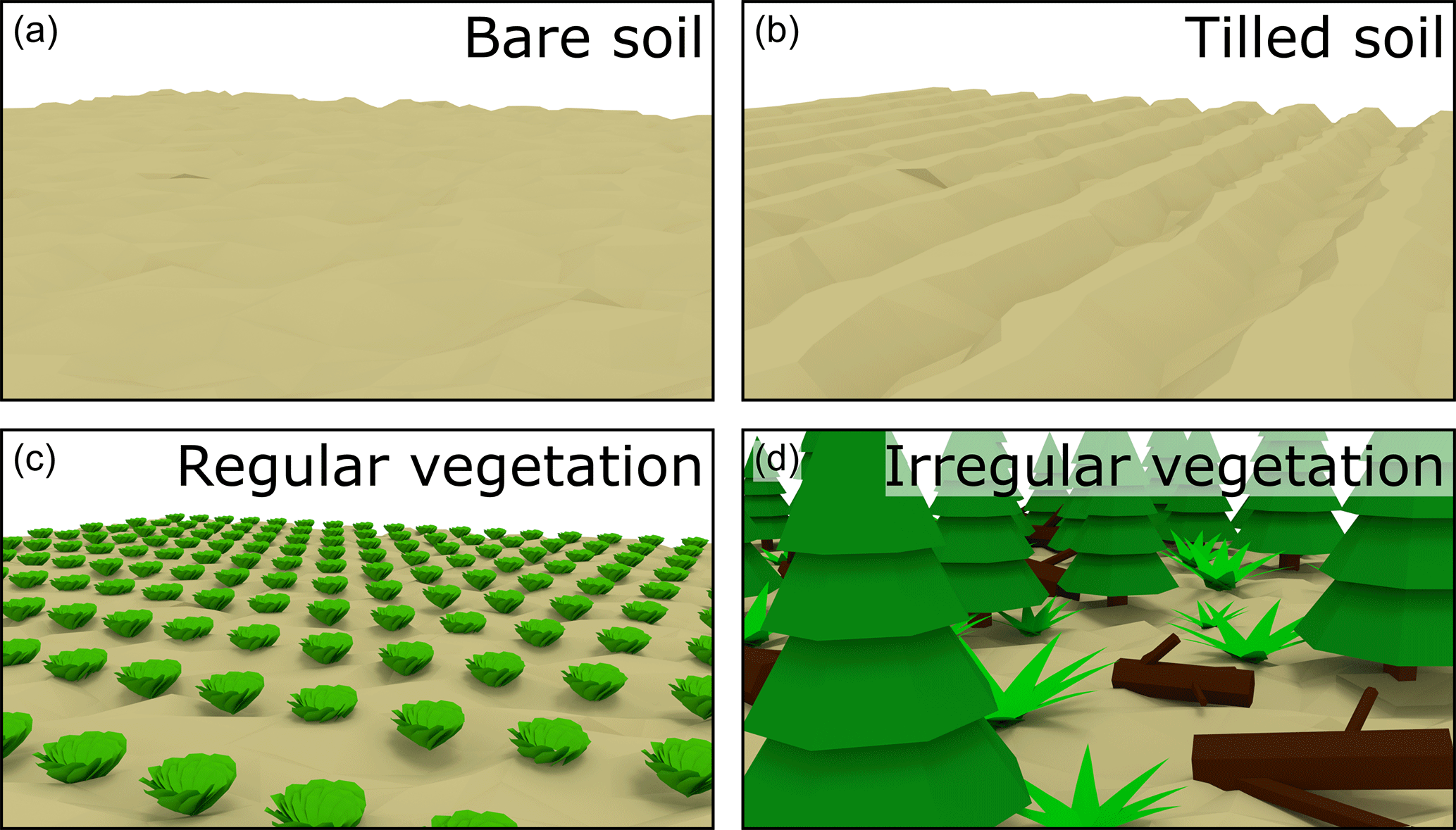
The Manning roughness coefficient for regularly spaced vegetation (nvegetation) (Fig. 2c) is obtained from the following equation (Jin et al., 2000):
where D is the stem diameter (m) and NV is the stem density (stems m−2). Stem diameter and stem density may be difficult to obtain for certain land use classes with irregularly spaced vegetation (e.g. forest, shrubland); therefore, users may opt to use tabular values for nvegetation, e.g. from Chow (1959) (Fig. 2d). Preliminary model runs showed that Eq. (26) results in unrealistically high flow velocity values for land use classes where the stem density is very low, such as in orchards. Therefore, in these conditions where the influence of vegetation on flow velocity is negligible, nvegetation can be set to zero.

Equations (21), (23), and (26) require a flow depth (d), which is a model parameter that can be used in the model calibration. The value for d should be taken such that it corresponds to a water depth from runoff generated within the cell margins, i.e. without accumulation of flow from upstream located cells.
2.3.4 Sediment deposition and transport
The amount of sediment that is routed to downstream cells is determined from the sum of the detached sediment from raindrop impact (Eq. 18) and accumulated runoff (Eq. 19), subtracting the proportion of the sediment that is deposited within the cell of its origin (Eq. 20):
The amount of sediment that is routed to downstream cells is the summation of the individual amounts for clay, silt, and sand.
Sediment is routed using a routing scheme that takes both the transport capacity (TC; ton ha−1) of the accumulated runoff and the trapping efficiency of the reservoirs (TE; –) into account. The transport capacity TC (Fig. 3a) of the accumulated runoff is based on Prosser and Rustomji (2000):
where flowfactor is a spatially distributed roughness factor (–), qsurf is accumulated runoff per unit width (m2 day−1), S is the local energy gradient (∘), approximated by the slope, and β and γ are model parameters (–). As suggested by Prosser and Rustomji (2000), γ is set to 1.4 and β is used for model calibration.
The roughness factor (flowfactor) is determined as follows:
where vactual is the actual flow velocity (m s−1) and vbare is the flow velocity for bare soil conditions (m s−1). The actual flow velocity (vactual) is obtained from Eqs. (23)–(26), applying a water depth (dactual) of 0.25 m, which coincides with deeper rills from Morgan and Duzant (2008). The flow velocity for bare soil conditions (vbare) is obtained from Eq. 23, applying values for s m and dbare=0.005 m (Morgan and Duzant, 2008).
Reservoir sediment trapping efficiency (TE) (Fig. 3b), the percentage of sediment trapped by the reservoir, is calculated according to Brown (1943):
where D is a constant (–) within the range from 0.046 to 1, depending on the reservoir operation characteristics that we set at 0.1, C is the reservoir capacity (m3), and Abasin is the drainage area of the subcatchment (km2).
To illustrate the model performance, its functionality, and its capacity for use in scenario studies, we applied the model to the upper Segura River catchment (2589 km2) under present and future projected climate conditions. The upper Segura catchment is located in the headwaters of the Segura River in southeastern Spain (Fig. 4). The elevation ranges between 411 and 2055 m a.s.l. (Fig. 4). The climate in the catchment is classified as temperate (Cfa and Cfb according to the Köppen–Geiger climate classification, 80 %) and semi-arid (BSk, 20 %). The catchment-average annual precipitation is 570 mm (for the period from 1981 to 2000) and the mean annual temperature is 13.2 ∘C (for the period from 1981 to 2000).
The main land use types are forest (45 %), shrubland (40 %), cereal fields (7 %), and almond orchards (4 %) (Fig. 4), based on a detailed land use map (MAPAMA, 2010). Agriculture accounts for 14 % of the catchment's surface area. Huerta is defined as small-scale traditional vegetable and/or fruit orchards, which are common in the study area. The main soil classes are Leptosols (38 %), Luvisols (27 %), Cambisols (16 %), and Calcisols (11 %), based on the SoilGrids database (Hengl et al., 2017). There are five reservoirs located in the catchment (Fig. 4b) with a total capacity of 663 Hm3, which are mainly used to store water for irrigation purposes.
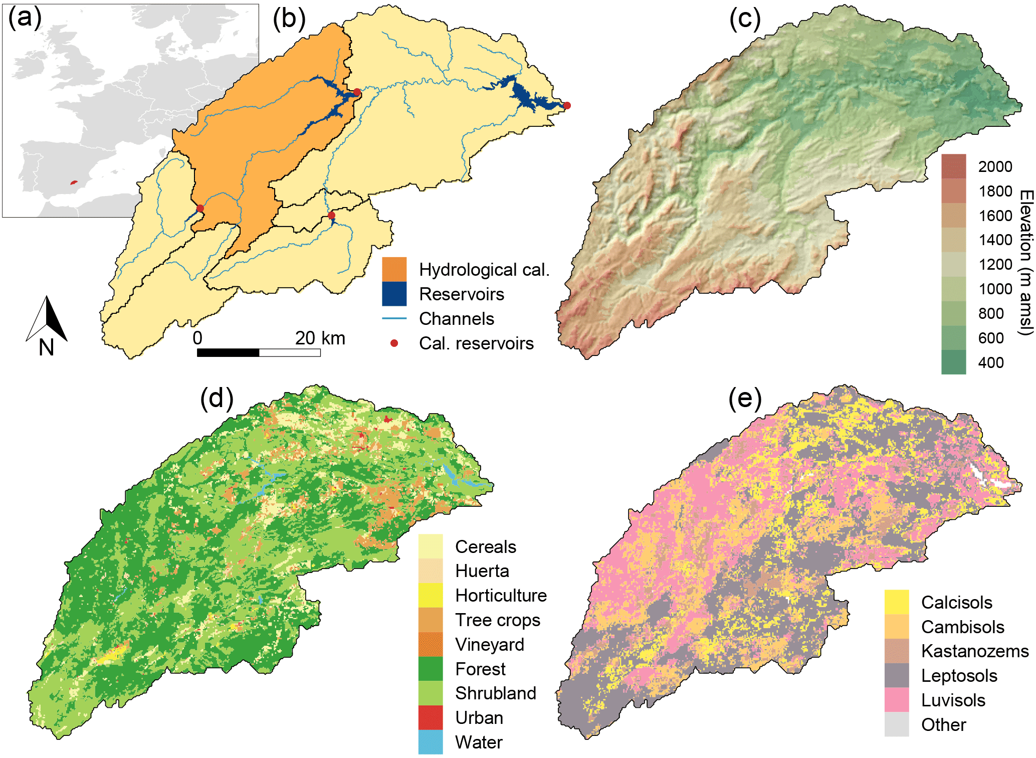
Figure 4Location and characteristics of the upper Segura River catchment: (a) location of the catchment within Europe; (b) the hydrological calibration area (orange), the channels (light blue), the reservoirs (dark blue), and the calibration reservoirs (red dots); (c) digital elevation model (Farr et al., 2007); (d) land use map (MAPAMA, 2010); and (e) soil texture map (Hengl et al., 2017).
3.1 Input data
All input data were prepared at a 200 m grid size. Daily precipitation data were obtained from the SPREAD dataset (Serrano-Notivoli et al., 2017), with a 5 km spatial resolution. Daily temperature data were obtained from the Spain02 dataset (Herrera et al., 2016), with a 0.11∘ resolution. Precipitation and temperature data were subsequently interpolated on the model grid using bivariate interpolation (Akima, 1996). Soil textural fractions (sand, clay, and silt) and soil organic matter content were obtained from the global SoilGrids dataset (Hengl et al., 2017) at 250 m resolution. The soil hydraulic properties (saturated hydraulic conductivity, saturated water content, field capacity, and wilting point) were obtained by applying pedotransfer functions (Saxton and Rawls, 2006). A digital elevation model was obtained from the SRTM dataset (Farr et al., 2007) at 30 m resolution and was resampled to the model grid using bilinear interpolation (Fig. 4d). The spatially distributed rock fraction map was obtained by applying the empirical formulations from Poesen et al. (1998), which determine rock fraction based on slope gradient.
Table 1Input parameters for the soil erosion model.
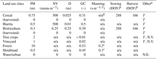
a T represents tillage, N.E. represents no erosion, N.V. represents no vegetation, b day of the year, c obtained from Chow (1959), and d not applicable.
Both the hydrological and the soil erosion model require land use specific input. We used a detailed land use map (MAPAMA, 2010) that identifies 25 land use classes within the study area. Values for the land use specific tabular value of the depletion fraction (ptabular) to calculate actual evapotranspiration were obtained from Table 22 in Allen et al. (1998). Values for the maximum LAI (LAImax) were obtained from Sellers et at. (1996). The soil erosion model requires land use specific input for plant height (PH), stem density (NV), stem diameter (D), ground cover fraction (GC) and, optionally, the Manning roughness coefficient for vegetation (nvegetation). The user needs to specify whether the land use class is non-erodible (e.g. pavement and water), tilled, or non-vegetated (e.g. bare soil or tilled orchards). We obtained values for each of these parameters through observations from aerial photographs, expert judgement, and as part of the calibration procedure (Table 1). The tillage parameter RFR was set to six, which corresponds to “Cultivator tillage” in Table 4 of Morgan and Duzant (2008). The input parameters change when a crop is harvested; therefore, we varied the input parameters according to the sowing–harvest cycle representing the cropping cycle for horticulture and cereals. Table 1 shows the values of all the land use specific input parameters after calibration.
We applied the dynamic vegetation module to obtain crop coefficients and vegetation cover from NDVI, which we obtained from the 16-day Moderate Resolution Imaging Spectroradiometer data (Didan, 2015) for the period from 2000 to 2012. For model calibration (2001–2010) we used each of the individual NDVI images, after gap-filling (mainly due to cloud cover) with the long-term average 16-day period NDVI for the period from 2000 to 2012.
For the model validation period (1981–2000) no NDVI images of sufficient quality and resolution were available; therefore, we prepared NDVI model input accounting for the intra- and inter-annual variability. The intra-annual variability was obtained from the long-term average 16-day period NDVI for the period from 2000 to 2012. The inter-annual variability was determined based on a log-linear relationship between the annual precipitation sum, annual mean temperature, annual maximum temperature, and yearly averaged NDVI for each of the 25 land use classes for the period from 2000 to 2012:
where NDVI is the yearly averaged NDVI, P is the annual precipitation sum, Tavg is the annual mean temperature, Tmax is the annual maximum temperature, and β0−6 are coefficients of the log-linear model. We used the annual climate indices of two years, the current year, and the previous year, to account for the climate lag that may influence the vegetation development. A stepwise model selection procedure was applied for each of the 25 land use classes, selecting the best combination of variables from Eq. (31) with the lowest AIC (Akaike information criterion) in R (version 3.4.0), using the stepAIC algorithm from the MASS package (Venables and Ripley, 2002).
3.2 Model calibration & validation
We calibrated the model for the period from 2001 to 2010. To prevent overfitting and achieve the most realistic model calibration we set most of the potential calibration parameters at literature values and maintained the other parameters within reasonable physical limits of the parameter domain. We used daily discharge time series from the Segura River Basin Agency (Confederación Hidrográfica del Segura) for the Fuensanta Reservoir (Fig. 4b) to determine model performance for the hydrological model. The calibration procedure consisted of two steps. Firstly, we optimized by minimising the difference between the observed and simulated discharge sum at the Fuensanta discharge station. We adjusted the calibration parameter λ from Eq. 6 to obtain a surface runoff ratio between 2 and 10 %, which previous studies reported to be representative for catchments with similar conditions (Descroix et al., 2001; Love et al., 2010; Mekki et al., 2006; Reaney et al., 2014). We used parameters from the dynamic vegetation module and soil hydraulic properties to optimise the difference in discharge sum (percent bias). Secondly, using the parameter set from the first step, we optimized the Nash–Sutcliffe model efficiency (Nash and Sutcliffe, 1970) at the Fuensanta discharge station by calibrating the routing parameter (kx). The calibration resulted in a NSE of 0.47 for the daily discharge data, a NSE of 0.76 for the monthly discharge data, and a percent bias of 2.3 % (Fig. 5a). Model validation for the period from 1981 to 2000 resulted in a NSE of 0.25 for the daily discharge data, a NSE of 0.39 for the monthly discharge data, and a percent bias of −18.7 % (5b). These model efficiency values are similar to previous SPHY model applications (Terink et al., 2015).
Cerdan et al. (2010)Maetens et al. (2012)Table 2Calibration and validation of hillslope soil erosion and comparison with literature data (Mg km−2 yr−1), where NA stands for not available.
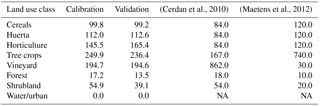
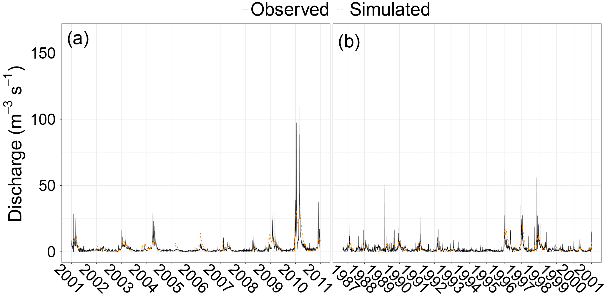
Figure 5Discharge time series for the calibration (a) and validation period (b). The solid line corresponds to the observed time series and the dashed orange line corresponds to the simulated time series.
To calibrate the soil erosion model we first optimized the detached material going into transport (G) for 8 land use classes (aggregated from 25 land use classes), based on literature data (Cerdan et al., 2010; Maetens et al., 2012) (Table 2). The resulting optimized parameter values are presented in Table 1. Next, we optimized percent bias in the prediction of sediment yield at the reservoirs using measured reservoir sediment yield data from four reservoirs (Avendaño-Salas et al., 1997). Annual sediment yield at the reservoirs was determined from the measured reservoir volume at two moments in time and the measured bulk density. Figure 4b shows the locations of the reservoirs used for calibration. The calibration procedure focused on the most sensitive parameter from the sediment transport capacity equation (Eq. 28), i.e. the β parameter. We obtained a percent bias of 0.0 % in the calibration and −19.8 % in the validation (see Fig. 6).
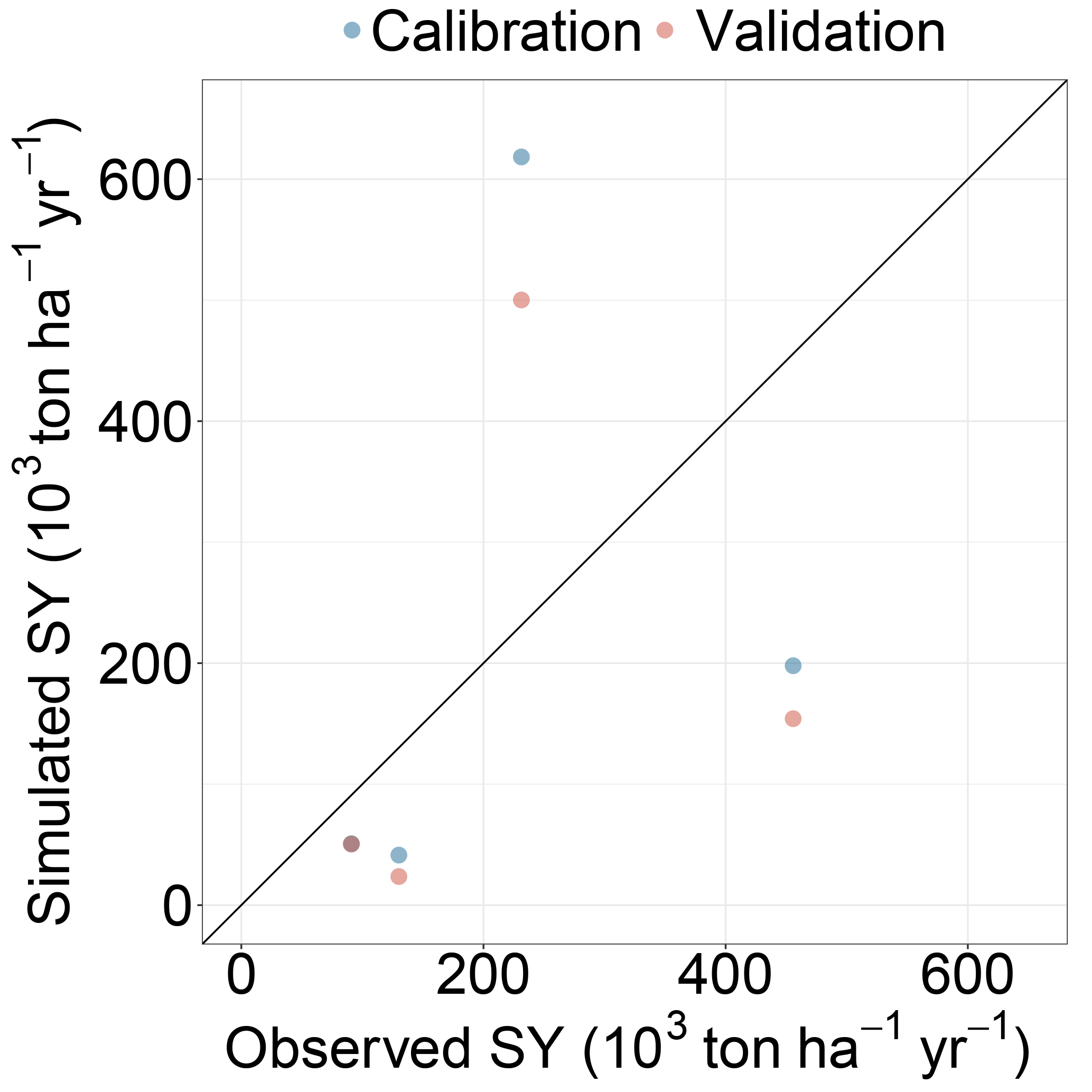
Figure 6Average yearly sediment yield (SY) at the reservoirs for the calibration (blue) and validation period (red).
3.3 Results
Here we present a selection of model results to illustrate the main capabilities of the SPHY–MMF model. Soil erosion shows an important intra-annual variability due to seasonal changes in climate forcing and vegetation cover (Fig. 7). For crops with little to no ground cover (i.e. tree crops and vineyard), soil erosion follows the precipitation sum, with high values in the winter, spring, and autumn months and low values in the summer months. Some crops show a distinct peak in the vegetation development in the spring (April–May), e.g. huerta and horticulture. While this period has a relatively high precipitation sum, soil erosion decreases as a consequence of the increased vegetation cover indicated by the NDVI in this period.
The temporal variation of the vegetation development of cereals and horticulture shows a slightly distinct pattern from the other land use classes. Both crops show an increase in the spring months (March–May), which indicates the rapid growth of these crops in these months. However, during the summer months (June–August) the NDVI decreases, which coincides with the period when the crops are harvested, followed by the post-harvest period. In the latter period, we assume bare soil conditions for these crops. For both crops this ultimately results in the highest annual erosion rates in the post-harvest period (October).
To illustrate the models capacity to perform scenario studies we evaluated the impacts of the application of sustainable land management and the impacts of a future climate change scenario. First, we evaluated the application of a sustainable land management scenario in cereal and horticulture fields. We assumed that after harvest the cereal and horticulture fields are not tilled until the next sowing. We parameterized this by setting the plant height to zero and leaving all other input parameters unchanged, i.e. stem density, diameter and ground cover, which in the conventional scenario are also set to zero. This will affect immediate deposition of detached particles through Eq. (26). The sustainable land management scenario leads to lower soil erosion estimates for these two land use classes (dashed lines in Fig. 7), as a result of an increase of immediate deposition of detached particles.
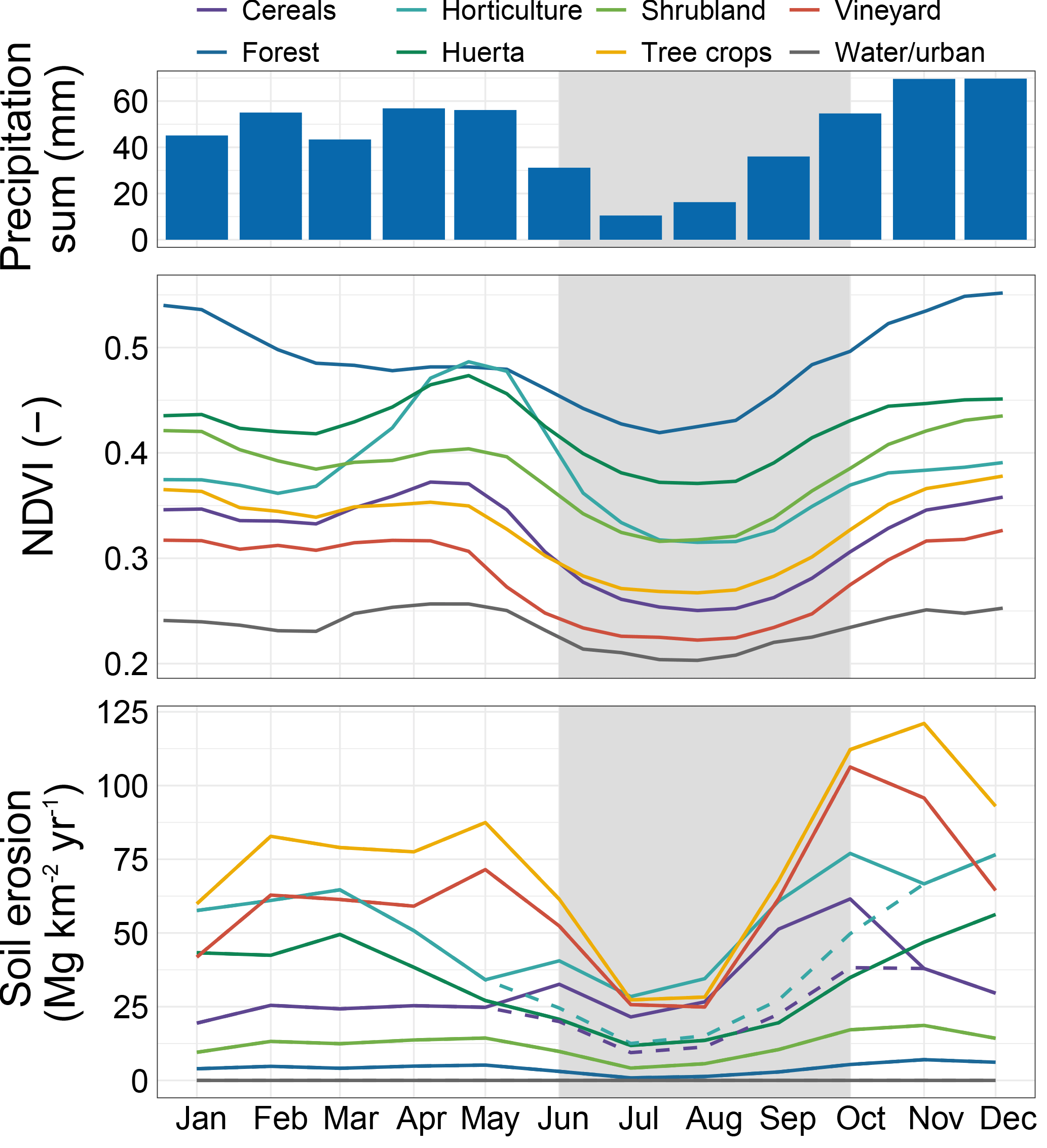
Figure 7Monthly precipitation sum (mm), NDVI (–), and soil erosion (Mg km−2 yr−1) per land use class for the period from 1981 to 2000. The gray area indicates the period when cereals and horticulture are harvested and model parameters are changed to simulate bare soil conditions. The dashed lines in the lower panel show the soil erosion of cereals and horticulture under the sustainable land management scenario.
Next, we simulated the impacts of a projected climate change scenario, by comparing predicted soil erosion rates and sediment yield under the reference scenario (1981–2000) with a future scenario (2081–2100). We used a future emission scenario from the Representative Concentration Pathways (van Vuuren et al., 2011) that describes a continuous increase of GHG emissions throughout the 21st century, i.e. RCP8.5. For this exercise we used projected climate data for RCP8.5 obtained from a regional climate model (CLMcom MPI-ESM-LR) from the EURO-CORDEX initiative (Jacob et al., 2014), for the period from 2081 to 2100. The climate forcing (precipitation and temperature) was bias-corrected using quantile mapping (Themeßl et al., 2012) and we applied the log-linear relationship (Eq. 31) to construct future NDVI input based on future climate conditions. Figure 8 shows the precipitation and vegetation response under the reference and future scenarios. The annual precipitation sum decreases in the future scenario, with a catchment-averaged decrease of 128 mm. However, heavy precipitation, defined as the 95th percentile of daily precipitation, considering only rainy days (Jacob et al., 2014), increases by 27 % on average in the catchment. The NDVI increases in the western part of the catchment due to increasing temperatures and decreases in the eastern part of the catchment due to a combination of decreasing precipitation and increasing temperatures.
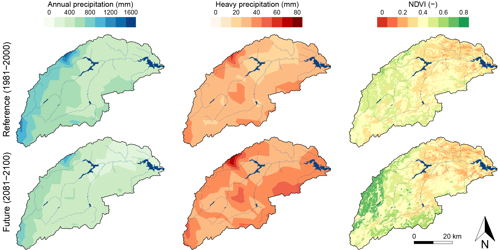
Figure 8Average annual precipitation sum (mm), heavy precipitation (mm), and NDVI (–) for the reference (1981–2000) and future (2081–2100) scenarios.
In the reference scenario the highest specific sediment yield (SSY) is projected in the river network (Fig. 9), where accumulated runoff causes an increase of soil erosion rates (Eq. 19). In the future climate scenario, the catchment-median SSY increases from 43.3 to 55.2 Mg km−2 yr−1, an increase of 27.7 %. This shows that the increase in heavy precipitation has a more pronounced impact on soil erosion than the decrease of annual precipitation sum. The increase of heavy precipitation leads to both an increase of detachment by raindrop impact (Eq. 18) and an increase of detachment by runoff (Eq. 19), as a consequence of an increase in surface runoff due to infiltration excess surface runoff. However, as a result of the increased vegetation cover in the western part of the catchment SSY decreases, despite the increased extreme precipitation intensities (Fig. 8).
Reservoir sediment yield (SY) decreases in all five reservoirs between 42.4 % and 59.0 % in the future climate scenario. While it is likely that a decrease of SSY in the western part of the catchment causes a decrease of reservoir SY, it is less obvious why in the eastern part of the catchment an increase in SSY is not reflected in an increase in reservoir SY. The explanation for this lies in the fact that a decrease in precipitation sum causes a decrease of accumulated runoff and, subsequently, a decrease of sediment transport capacity (Eq. 28), increased sediment deposition, and decreased reservoir SY.
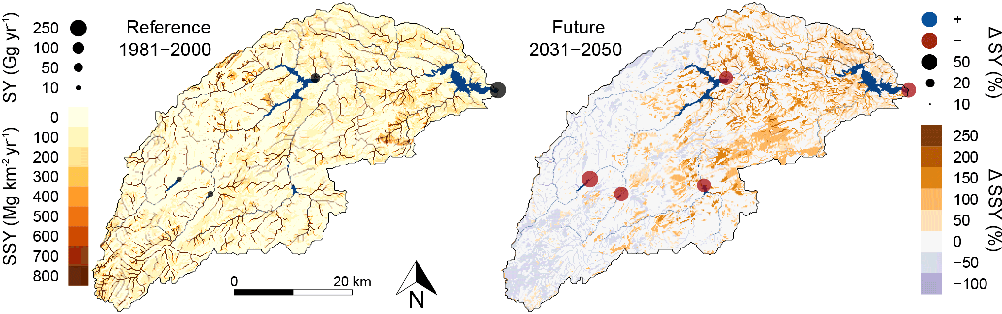
Figure 9Specific sediment yield (Mg km−2 yr−1) and reservoir sediment yield (Gg yr−1) for the reference (1981–2000) scenario and the change (%) for the future (2081–2100) scenario.
The SPHY–MMF model, based on integration of the SPHY hydrological model with the MMF soil erosion model, provides an important step toward simulating the regional scale impacts of environmental change on soil erosion and sediment yield. The processes included in the model provide the flexibility and accuracy needed to reflect the impacts of intra-annual changes in land use, land management and climate (Fig. 7), and the inter-annual response of vegetation development and soil erosion to changes in climate forcing, including changes in precipitation sum and intensity (Fig. 9).
The availability of high quality input data and model parameter values are important constraints for many process-based soil erosion models. Although SPHY–MMF requires a wide range of input data, most data were obtained from publicly available global datasets at relatively high spatial and temporal resolution. Whilst climate data may often be an important constraint, long-term, high-resolution, gridded daily climate forcing datasets are becoming increasingly available at national (Berezowski et al., 2016; Kotlarski et al., 2017; Silva et al., 2007; Yin et al., 2015), (sub-)continental (Haylock et al., 2008; Mitchell, 2004; Yatagai et al., 2012; van den Besselaar et al., 2017), and even global scales (Donat et al., 2013; Huffman et al., 2001; Schamm et al., 2016). Although, the model includes a large number of parameters (Table S1), we do not expect this to limit the model's applicability. Apart from the land use specific parameters, all soil erosion model parameters were obtained from the literature, mainly from Morgan and Duzant (2008). Although some parameters may be obtained from calibration, the possibility to use literature values facilitates model application. The model requires a detailed land use map to account for land use specific model parameters that drive soil erosion processes (Table S1), which may be inevitable because soil erosion is inherently land use dependent. For example, we obtained literature values for five land use related model parameters (Table S1), while others were obtained through observations from aerial photographs, expert judgement, and as part of the calibration procedure. The ground cover for cereals, for instance, was obtained by adjusting the stem density, assuming a certain ground cover per stem. Most other input datasets are publicly available and most model parameters may be obtained from literature, which makes the model applicable for any environment.
One of the main limitations of the model is that unrealistic high soil erosion rates are projected where most flow accumulates (Fig. 9). This is mainly due to the high amounts of soil erosion predicted by Eq. (19) for large runoff volumes. Similar behaviour was reported in a daily implementation of the MMF model by Shrestha and Jetten (2018), who subsequently suggested excluding higher order streams from the soil erosion assessment. We correct for the high erosion rates in the river network by including both immediate sediment deposition (Eq. 20) and deposition when the transport capacity is exceeded (Eq. 28). While different erosional processes indeed dominate in channels and streams (i.e. bank erosion and channel incision), which are not captured by Eq. (19), high soil erosion rates may be expected in the river network since many studies stress the large contribution of gully and channel erosion to total sediment yield due to large volumes of accumulated runoff (Poesen, 2018; Poesen et al., 1996; Vanmaercke et al., 2011; de Vente et al., 2008). However, detachment and transport processes in channels are likely different from those on hillslopes and the bed material of rivers differs from the soil texture as used in the model. While Eq. (19) makes a distinction between the three textural classes, it most likely overestimates the erosion in the higher order channels, where in reality the bed material consists of coarser material, such as coarse sand and gravel, which is currently not included in the model. Therefore, in a future update of the model, we suggest the inclusion of a separate channel model to simulate the most relevant channel erosion, transport, and deposition processes more accurately. Recently, several models have been proposed that incorporate fluvial processes into soil erosion models (Arnold et al., 2012; Wei et al., 2017) and landscape evolution models (Baartman et al., 2012; Coulthard et al., 2013), which could serve as a starting point for further model development.
The model is intended to be applied at regional scales and over decadal periods that are most relevant for policy makers. This poses some limitations to the spatial and temporal representation of some essential soil erosion processes. Firstly, the spatial resolution of the model is bounded by the hydrological model. Each cell generates runoff, which is a composite of surface runoff, lateral flow, and base flow (Fig. 1b). Lateral flow and base flow are generally only generated at large spatial scales, imposing a lower limit for the spatial resolution. Therefore, Terink et al. (2015) suggests a spatial resolution in the range of 200 m to 1 km. The lower limit of the spatial resolution may affect the simulation of soil erosion processes. For instance, the detachment of soil particles by runoff is determined by slope, among other variables. The lower limit of the spatial resolution may result in a flattening of the digital elevation model, especially affecting steep slopes. Ultimately, this results in lower soil erosion projections on the most extreme slopes. Secondly, the daily time step limits the simulation of high intensity (sub-)hourly rain storms, which often cause the most soil erosion (Nearing et al., 1990). Therefore, we included a model parameter (α) describing the relation between measured hourly and daily precipitation (see Eq. 8). Nevertheless, given the spatial scale at which the model is applied, running the model with (sub-)hourly time steps may still be infeasible for various reasons. At regional scales, (sub-)hourly precipitation data are often not available, while spatial interpolation of (sub-)hourly precipitation data may introduce large uncertainties, jeopardising the model outcome. Also, climate change assessments would become challenging, since most future climate model output is only available in daily time steps.
We have presented a new coupled hydrology, soil erosion, and sediment yield prediction model (SPHY–MMF), and its application to the upper Segura catchment for different climate and land management scenarios. The model is an integration of the MMF soil erosion model into the SPHY hydrological model and simulates most relevant hydrological and soil erosion processes at a daily time step. The model considers soil detachment by raindrop and runoff, uses dynamic vegetation to simulate changes in the canopy cover, simulates saturation excess and infiltration excess surface runoff, simulates soil deposition in the cell of its origin, and routes the sediment through the river network, considering the transport capacity of the flow. The model was successfully applied in a large catchment in southeastern Spain. We have shown that the model is capable of performing scenario assessments of changes in climate and land management. Furthermore, our results show that the model simulates the soil erosion response to intra-annual variability in climate conditions and vegetation development. While multiple challenges to accurately simulating the impacts of environmental change on soil erosion and sediment yield remain, we consider the integrated SPHY–MMF model an important step toward facilitating catchment-scale scenario studies.
The model source code is available online: https://doi.org/10.5281/zenodo.1344534 (Eekhout et al., 2018).
The supplement related to this article is available online at: https://doi.org/10.5194/esurf-6-687-2018-supplement.
JPCE, WT and JdV developed the model, JPCE and JdV applied the model, and JPCE wrote the paper with contributions from the other authors.
The author declares that they have no conflict of interest.
We acknowledge financial support from the “Juan de la Cierva” program of the
Spanish Ministerio de Economía y Competitividad (FJCI-2016-28905), the
Spanish Ministerio de Economía y Competitividad (ADAPT project;
CGL2013-42009-R), and the Séneca foundation of the regional government of
Murcia (CAMBIO project; 118933/JLI/13). The authors thank AEMET and UC for
the data provided for this work (the Spain02 v5 dataset is available at:
http://www.meteo.unican.es/datasets/spain02).
Edited by: Greg Hancock
Reviewed by: Arnaud Temme and Agustin Millares
Abrahams, A. D., Li, G., Krishnan, C., and Atkinson, J. F.: A sediment transport equation for interrill overland flow on rough surfaces, Earth Surf. Proc. Land., 26, 1443–1459, https://doi.org/10.1002/esp.286, 2001. a
Akima, H.: Algorithm 761; scattered-data surface fitting that has the accuracy of a cubic polynomial, ACM T. Math. Software, 22, 362–371, https://doi.org/10.1145/232826.232856, 1996. a
Allen, R. G., Pereira, L., Raes, D., and Smith, M.: Crop evapotranspiration: Guidelines for computing crop requirements, Tech. Rep., 56, https://doi.org/10.1016/j.eja.2010.12.001, 1998. a
Arnold, J. G., Moriasi, D. N., Gassman, P. W., Abbaspour, K. C., White, M. J., Srinivasan, R., Santhi, C., Harmel, R. D., Griensven, a. V., VanLiew, M. W., Kannan, N., and Jha, M. K.: Swat: Model Use, Calibration, and Validation, Asabe, 55, 1491–1508, 2012. a
Avendaño-Salas, C., Sanz-Montero, E., Cobo-Rayán, R., and Gómez-Montaña, J. L.: Capacity Situation in Spanish Reservoirs, in: ICOLD, Proceedings of the 19th International Symposium on Large Dams, Florence, Italy, 849–862, 1997. a
Baartman, J. E. M., Gorp, W., Temme, A. J. A. M., and Schoorl, J. M.: Modelling sediment dynamics due to hillslope-river interactions: incorporating fluvial behaviour in landscape evolution model LAPSUS, Earth Surf. Proc. Land., 37, 923–935, https://doi.org/10.1002/esp.3208, 2012. a
Berezowski, T., Szcześniak, M., Kardel, I., Michalowski, R., Okruszko, T., Mezghani, A., and Piniewski, M.: CPLFD-GDPT5: High-resolution gridded daily precipitation and temperature data set for two largest Polish river basins, Earth Syst. Sci. Data, 8, 127–139, https://doi.org/10.5194/essd-8-127-2016, 2016. a
Beven, K. J.: Rainfall-runoff modelling: the primer, John Wiley & Sons, Ltd., Chichester, UK, https://doi.org/10.1002/9781119951001, 2012. a, b
Bouwer, H.: Infiltration of Water into Nonuniform Soil, J. Irr. Drain. Div.-ASCE, 95, 451–462, 1969.
Brandt, C. J.: Simulation of the size distribution and erosivity of raindrops and throughfall drops, Earth Surf. Proc. Land., 15, 687–698, https://doi.org/10.1002/esp.3290150803, 1990.
Brown, C. B.: Discussion of Sedimentation in reservoirs, T. Am. Soc. Civ. Eng., 69, 1493–1500, 1943.
Burt, T., Boardman, J., Foster, I., and Howden, N.: More rain, less soil: long-term changes in rainfall intensity with climate change, Earth Surf. Proc. Land., 41, 563–566, https://doi.org/10.1002/esp.3868, 2016. a
Cerdan, O., Govers, G., Le Bissonnais, Y., Van Oost, K., Poesen, J., Saby, N., Gobin, A., Vacca, A., Quinton, J., Auerswald, K., Klik, A., Kwaad, F. J. P. M., Raclot, D., Ionita, I., Rejman, J., Rousseva, S., Muxart, T., Roxo, M. J., and Dostal, T.: Rates and spatial variations of soil erosion in Europe: A study based on erosion plot data, Geomorphology, 122, 167–177, https://doi.org/10.1016/j.geomorph.2010.06.011, 2010. a, b
Choi, K., Arnhold, S., Huwe, B., and Reineking, B.: Daily Based Morgan-Morgan-Finney (DMMF) Model: A Spatially Distributed Conceptual Soil Erosion Model to Simulate Complex Soil Surface Configurations, Water, 9, 278, https://doi.org/10.3390/w9040278, 2017. a
Chow, V. T.: Open-Channel Hydraulics, McGraw-Hill Book Company, New York, USA, ISBN 07-010776-9, 1959. a
Coulthard, T. J., Neal, J. C., Bates, P. D., Ramirez, J., de Almeida, G. a. M., and Hancock, G. R.: Integrating the LISFLOOD-FP 2D hydrodynamic model with the CAESAR model: Implications for modelling landscape evolution, Earth Surf. Proc. Land., 38, 1897–1906, https://doi.org/10.1002/esp.3478, 2013. a
de Vente, J., Poesen, J., Arabkhedri, M., and Verstraeten, G.: The sediment delivery problem revisited, Prog. Phys. Geog., 31, 155–178, https://doi.org/10.1177/0309133307076485, 2007. a
de Vente, J., Poesen, J., Verstraeten, G., Van Rompaey, A., and Govers, G.: Spatially distributed modelling of soil erosion and sediment yield at regional scales in Spain, Global Planet. Change, 60, 393–415, https://doi.org/10.1016/j.gloplacha.2007.05.002, 2008. a, b
de Vente, J., Poesen, J., Verstraeten, G., Govers, G., Vanmaercke, M., Van Rompaey, A., Arabkhedri, M., and Boix-Fayos, C.: Predicting soil erosion and sediment yield at regional scales: Where do we stand?, Earth-Sci. Rev., 127, 16–29, https://doi.org/10.1016/j.earscirev.2013.08.014, 2013. a, b, c
Descroix, L., Viramontes, D., Vauclin, M., Gonzalez Barrios, J., and Esteves, M.: Influence of soil surface features and vegetation on runoff and erosion in the Western Sierra Madre (Durango, Northwest Mexico), CATENA, 43, 115–135, https://doi.org/10.1016/S0341-8162(00)00124-7, 2001. a
Didan, K.: MOD13Q1 MODIS/Terra Vegetation Indices 16-Day L3 Global 250m SIN Grid V006, https://doi.org/10.5067/modis/mod13q1.006, 2015. a, b
Donat, M. G., Alexander, L. V., Yang, H., Durre, I., Vose, R., Dunn, R. J. H., Willett, K. M., Aguilar, E., Brunet, M., Caesar, J., Hewitson, B., Jack, C., Klein Tank, A. M. G., Kruger, A. C., Marengo, J., Peterson, T. C., Renom, M., Oria Rojas, C., Rusticucci, M., Salinger, J., Elrayah, A. S., Sekele, S. S., Srivastava, A. K., Trewin, B., Villarroel, C., Vincent, L. A., Zhai, P., Zhang, X., and Kitching, S.: Updated analyses of temperature and precipitation extreme indices since the beginning of the twentieth century: The HadEX2 dataset, J. Geophys. Res.-Atmos., 118, 2098–2118, https://doi.org/10.1002/jgrd.50150, 2013. a
Eekhout, J. P. C. and De Vente, J.: SPHY-MMF – Coupled Hydrology-Soil Erosion Model (video abstract), https://doi.org/10.5446/37585, 2018.
Eekhout, J. P. C., Terink, W., and De Vente, J.: SPHY-MMF – Coupled Hydrology-Soil Erosion Model, https://doi.org/10.5281/zenodo.1344534, 2018.
Farnsworth, K. L. and Milliman, J. D.: Effects of climatic and anthropogenic change on small mountainous rivers: the Salinas River example, Global Planet. Change, 39, 53–64, https://doi.org/10.1016/S0921-8181(03)00017-1, 2003. a
Farr, T. G., Rosen, P. A., Caro, E., Crippen, R., Duren, R., Hensley, S., Kobrick, M., Paller, M., Rodriguez, E., Roth, L., Seal, D., Shaffer, S., Shimada, J., Umland, J., Werner, M., Oskin, M., Burbank, D., and Alsdorf, D.: The Shuttle Radar Topography Mission, Rev. Geophys., 45, RG2004, https://doi.org/10.1029/2005RG000183, 2007. a, b
González-Hidalgo, J. C., Peña-Monné, J. L., and de Luis, M.: A review of daily soil erosion in Western Mediterranean areas, CATENA, 71, 193–199, https://doi.org/10.1016/j.catena.2007.03.005, 2007. a
González-Hidalgo, J. C., Batalla, R. J., Cerda, A., and de Luis, M.: A regional analysis of the effects of largest events on soil erosion, CATENA, 95, 85–90, https://doi.org/10.1016/j.catena.2012.03.006, 2012. a
Govers, G.: Misapplications and Misconceptions of Erosion Models, in: Handbook of Erosion Modelling, edited by: Morgan, R. P. C. and Nearing, M. A., John Wiley & Sons, Ltd, Chichester, UK, 117–134, https://doi.org/10.1002/9781444328455.ch7, 2011. a, b
Hargreaves, G. H. and Samani, Z. A.: Reference crop evapotranspiration from temperature, Appl. Eng. Agric., 1, 96–99, 1985. a
Haylock, M. R., Hofstra, N., Klein Tank, A. M. G., Klok, E. J., Jones, P. D., and New, M.: A European daily high-resolution gridded data set of surface temperature and precipitation for 1950–2006, J. Geophys. Res.-Atmos., 113, D20119, https://doi.org/10.1029/2008JD010201, 2008. a
Heber Green, W. and Ampt, G. A.: Studies on Soil Phyics, J. Agr. Sci., 4, 1–24, https://doi.org/10.1017/S0021859600001441, 1911. a, b
Hengl, T., Mendes de Jesus, J., Heuvelink, G. B. M., Ruiperez Gonzalez, M., Kilibarda, M., Blagotić, A., Shangguan, W., Wright, M. N., Geng, X., Bauer-Marschallinger, B., Guevara, M. A., Vargas, R., MacMillan, R. A., Batjes, N. H., Leenaars, J. G. B., Ribeiro, E., Wheeler, I., Mantel, S., and Kempen, B.: SoilGrids250m: Global gridded soil information based on machine learning, PLOS ONE, 12, e0169748, https://doi.org/10.1371/journal.pone.0169748, 2017. a, b, c
Herrera, S., Fernández, J., and Gutiérrez, J. M.: Update of the Spain02 gridded observational dataset for EURO-CORDEX evaluation: assessing the effect of the interpolation methodology, Int. J. Climatol., 36, 900–908, https://doi.org/10.1002/joc.4391, 2016. a
Huffman, G. J., Adler, R. F., Morrissey, M. M., Bolvin, D. T., Curtis, S., Joyce, R., McGavock, B., and Susskind, J.: Global Precipitation at One-Degree Daily Resolution from Multisatellite Observations, J. Hydrometeorol., 2, 36–50, https://doi.org/10.1175/1525-7541(2001)002<0036:GPAODD>2.0.CO;2, 2001. a
Jacob, D., Petersen, J., Eggert, B., Alias, A., Christensen, O. B., Bouwer, L. M., Braun, A., Colette, A., Déqué, M., Georgievski, G., Georgopoulou, E., Gobiet, A., Menut, L., Nikulin, G., Haensler, A., Hempelmann, N., Jones, C., Keuler, K., Kovats, S., Kröner, N., Kotlarski, S., Kriegsmann, A., Martin, E., van Meijgaard, E., Moseley, C., Pfeifer, S., Preuschmann, S., Radermacher, C., Radtke, K., Rechid, D., Rounsevell, M., Samuelsson, P., Somot, S., Soussana, J.-F., Teichmann, C., Valentini, R., Vautard, R., Weber, B., and Yiou, P.: EURO-CORDEX: new high-resolution climate change projections for European impact research, Reg. Environ. Change, 14, 563–578, https://doi.org/10.1007/s10113-013-0499-2, 2014. a, b
Jin, C. X., Römkens, J. M., and Griffioen, F.: Estimating manning's roughness coefficient for shallow overland flow in non-submerged vegetative filter strips, T. ASAE, 43, 1459–1466, 2000. a
Karssenberg, D., Schmitz, O., Salamon, P., de Jong, K., and Bierkens, M. F.: A software framework for construction of process-based stochastic spatio-temporal models and data assimilation, Environ. Modell. Softw., 25, 489–502, https://doi.org/10.1016/j.envsoft.2009.10.004, 2010. a, b
Kirkby, M.: Hillslope runoff processes and models, J. Hydrol., 100, 315–339, https://doi.org/10.1016/0022-1694(88)90190-4, 1988. a
Kotlarski, S., Szabó, P., Herrera, S., Räty, O., Keuler, K., Soares, P. M., Cardoso, R. M., Bosshard, T., Pagé, C., Boberg, F., Gutiérrez, J. M., Isotta, F. A., Jaczewski, A., Kreienkamp, F., Liniger, M. A., Lussana, C., and Pianko-Kluczyńska, K.: Observational uncertainty and regional climate model evaluation: a pan-European perspective, Int. J. Climatol., https://doi.org/10.1002/joc.5249, 2017. a
Li, K. Y., De Jong, R., Coe, M. T., and Ramankutty, N.: Root Water Uptake Based upon a New Water Stress Reduction and an Asymptotic Root Distribution Function, Earth Interact., 10, 1–22, https://doi.org/10.1175/EI177.1, 2006. a
López-Bermúdez, F., Conesia-García, C., and Alonso-Sarria, F.: Floods: Magnitude and frequency in ephemeral streams of the Spanish Mediterranean region, in: Dryland rivers, Hydrology and geomorphology of semi-arid channels, edited by: Bull, L. and Kirkby, M., John Wiley & Sons, Chichester, UK, 329–350, 2002. a
Love, D., Uhlenbrook, S., Corzo-Perez, G., Twomlow, S., and van der Zaag, P.: Rainfall-interception-evaporation-runoff relationships in a semi-arid catchment, northern Limpopo basin, Zimbabwe, Hydrolog. Sci. J., 55, 687–703, https://doi.org/10.1080/02626667.2010.494010, 2010. a
Maetens, W., Vanmaercke, M., Poesen, J., Jankauskas, B., Jankauskiene, G., and Ionita, I.: Effects of land use on annual runoff and soil loss in Europe and the Mediterranean: A meta-analysis of plot data, Prog. Phys. Geog., 36, 599–653, https://doi.org/10.1177/0309133312451303, 2012. a, b, c
MAPAMA: Mapa de Cultivos y Aprovechamientos de España 2000-2010 (1 : 50 000), available at: http://www.magrama.gob.es/es/cartografia-y-sig/publicaciones/agricultura/mac_2000_2009.aspx (last access: 17 March 2017), 2010. a, b, c
Marshall, J. S. and Palmer, W. M. K.: The distribution of raindrops with size, J. Meteorol., 5, 165–166, https://doi.org/10.1175/1520-0469(1948)005<0165:TDORWS>2.0.CO;2, 1948.
Mekki, I., Albergel, J., Ben Mechlia, N., and Voltz, M.: Assessment of overland flow variation and blue water production in a farmed semi-arid water harvesting catchment, Phys. Chem. Earth, 31, 1048–1061, https://doi.org/10.1016/j.pce.2006.07.003, 2006. a
Mitchell, K. E.: The multi-institution North American Land Data Assimilation System (NLDAS): Utilizing multiple GCIP products and partners in a continental distributed hydrological modeling system, J. Geophys. Res., 109, D07S90, https://doi.org/10.1029/2003JD003823, 2004. a
Morgan, R. P. C.: Soil Erosion and Conservation, Blackwell Science Ltd, Malden, USA, 3rd edn., 2005. a, b, c, d
Morgan, R. P. C. and Duzant, J. H.: Modified MMF (Morgan–Morgan–Finney) model for evaluating effects of crops and vegetation cover on soil erosion, Earth Surf. Proc. Land., 33, 90–106, https://doi.org/10.1002/esp.1530, 2008. a, b, c, d
Morgan, R. P. C. and Nearing, M. A.: Handbook of Erosion Modelling, Blackwell Publishing Ltd., Chichester, UK, https://doi.org/10.1002/9781444328455, 2011. a
Morgan, R. P. C., Quinton, J. N., Smith, R. E., Govers, G., Poesen, J. W. A., Auerswald, K., Chisci, G., Torri, D., and Styczen, M. E.: The European Soil Erosion Model (EUROSEM): a dynamic approach for predicting sediment transport from fields and small catchments, Earth Surf. Proc. Land., 23, 527–544, https://doi.org/10.1002/(SICI)1096-9837(199806)23:6<527::AID-ESP868>3.0.CO;2-5, 1998. a, b
Mulligan, M.: Modelling the geomorphological impact of climatic variability and extreme events in a semi-arid environment, Geomorphology, 24, 59–78, https://doi.org/10.1016/S0169-555X(97)00101-3, 1998. a
Nash, J. E. and Sutcliffe, J. V.: River Flow Forecasting Through Conceptual Models Part I-a Discussion of Principles*, J. Hydrol., 10, 282–290, https://doi.org/10.1016/0022-1694(70)90255-6, 1970. a
Nearing, M., Deer-Ascough, L., and Laflen, J. M.: SENSITIVITY ANALYSIS OF THE WEPP HILLSLOPE PROFILE EROSION MODEL, T. ASAE, 33, 0839–0849, https://doi.org/10.13031/2013.31409, 1990. a
Nearing, M. A., Foster, G. R., Lane, L. J., and Finkner, S. C.: A Process-Based Soil Erosion Model for USDA-Water Erosion Prediction Project Technology, T. ASAE, 32, 1587–1593, https://doi.org/10.13031/2013.31195, 1989. a, b
Nearing, M. A., Pruski, F. F., and O'Neal, M. R.: Expected climate change impacts on soil erosion rates: A review, J. Soil and Water Conserv., 59, 43–50, http://www.jswconline.org/content/59/1/43.abstract, 2004. a
Petryk, S. and Bosmajian, G.: Analysis of flow through vegetation, J. Hydr. Eng. Div.-ASCE, 101, 871–884, 1975.
Poesen, J.: Soil erosion in the Anthropocene: Research needs, Earth Surf. Proc. Land., 43, 64–84, https://doi.org/10.1002/esp.4250, 2018. a, b
Poesen, J. W., Vandaele, K., and Wesemael, B. V. A. N.: Contribution of gully erosion to sediment production on cultivated lands and rangelands, in: Erosion and Sediment Yield: Global and Regional Perspectives, Proceedings of the Exeter Symposium, Exeter, UK, July 1996, IAHS Publ., 236, 251–266, 1996. a
Poesen, J. W., van Wesemael, B., Bunte, K., and Benet, A. S.: Variation of rock fragment cover and size along semiarid hillslopes: a case-study from southeast Spain, Geomorphology, 23, 323–335, https://doi.org/10.1016/S0169-555X(98)00013-0, 1998. a
Prosser, I. P. and Rustomji, P.: Sediment transport capacity relations for overland flow, Prog. Phys. Geog., 24, 179–193, https://doi.org/10.1177/030913330002400202, 2000.
Quansah, C.: Laboratory experimentation for the statistical derivation of equations for soil erosion modelling and soil conservation design, PhD thesis, http://ethos.bl.uk/OrderDetails.do?uin=uk.bl.ethos.337734, 1982.
Reaney, S. M., Bracken, L. J., and Kirkby, M. J.: The importance of surface controls on overland flow connectivity in semi-arid environments: results from a numerical experimental approach, Hydrol. Proc., 28, 2116–2128, https://doi.org/10.1002/hyp.9769, 2014. a
Renard, K. G., Foster, G. R., Weesies, G. A., McCool, D. K., and Yoder, D. C.: Predicting soil erosion by water: a guide to conservation planning with the Revised Universal Soil Loss Equation (RUSLE), Agricultural Handbook No. 703, U.S. Dept. of Agr., Washington DC , USA, p. 384, http://www.ars.usda.gov/SP2UserFiles/Place/64080530/RUSLE/AH_703.pdf, 1997. a
Rose, C. W., Williams, J. R., Sander, G. C., and Barry, D. A.: A Mathematical Model of Soil Erosion and Deposition Processes: I. Theory for a Plane Land Element1, Soil Sci. Soc. Am. J., 47, 991–995, https://doi.org/10.2136/sssaj1983.03615995004700050030x, 1983. a
Saxton, K. E. and Rawls, W. J.: Soil Water Characteristic Estimates by Texture and Organic Matter for Hydrologic Solutions, Soil Sci. Soc. Am. J., 70, 1569, https://doi.org/10.2136/sssaj2005.0117, 2006. a
Schamm, K., Ziese, M., Raykova, K., Becker, A., Finger, P., Meyer-Christoffer, A., and Schneider, U.: GPCC Full Data Daily Version 1.0: Daily Land-Surface Precipitation from Rain Gauges built on GTS based and Historic Data, https://doi.org/10.5065/D6V69GRT, 2016. a
Sellers, P. J., Tucker, C. J., Collatz, G. J., Los, S. O., Justice, C. O., Dazlich, D. A., and Randall, D. A.: A Revised Land Surface Parameterization (SiB2) for Atmospheric GCMS. Part II: The Generation of Global Fields of Terrestrial Biophysical Parameters from Satellite Data, J. Climate, 9, 706–737, https://doi.org/10.1175/1520-0442(1996)009<0706:ARLSPF>2.0.CO;2, 1996. a, b, c, d
Serrano-Notivoli, R., Beguería, S., Saz, M. Á., Longares, L. A., and de Luis, M.: SPREAD: a high-resolution daily gridded precipitation dataset for Spain – an extreme events frequency and intensity overview, Earth Syst. Sci. Data, 9, 721–738, https://doi.org/10.5194/essd-9-721-2017, 2017. a
Shrestha, D. P. and Jetten, V. G.: Modelling erosion on a daily basis, an adaptation of the MMF approach, Int. J. Appl. Earth. Obs., 64, 117–131, https://doi.org/10.1016/j.jag.2017.09.003, 2018.
Silva, V. B. S., Kousky, V. E., Shi, W., and Higgins, R. W.: An Improved Gridded Historical Daily Precipitation Analysis for Brazil, J. Hydrometeorol., 8, 847–861, https://doi.org/10.1175/JHM598.1, 2007. a
Terink, W., Lutz, A. F., Simons, G. W. H., Immerzeel, W. W., and Droogers, P.: SPHY v2.0: Spatial Processes in HYdrology, Geosci. Model Dev., 8, 2009–2034, https://doi.org/10.5194/gmd-8-2009-2015, 2015. a, b, c, d
Themeßl, M. J., Gobiet, A., and Heinrich, G.: Empirical-statistical downscaling and error correction of regional climate models and its impact on the climate change signal, Clim. Change, 112, 449–468, https://doi.org/10.1007/s10584-011-0224-4, 2012. a
Tollner, E. W., Barfield, B. J., Haan, C. T., and Kao, T. Y.: Suspended Sediment Filtration Capacity of Simulated Vegetation, T. ASAE, 19, 678–682, https://doi.org/10.13031/2013.36095, 1976.
van den Besselaar, E. J., van der Schrier, G., Cornes, R. C., Suwondo, A., Iqbal, and Tank, A. M.: SA-OBS: A daily gridded surface temperature and precipitation dataset for Southeast Asia, J. Climate, 30, 5151–5165, https://doi.org/10.1175/JCLI-D-16-0575.1, 2017. a
Van Rompaey, A. J. J., Verstraeten, G., Van Oost, K., Govers, G., and Poesen, J.: Modelling mean annual sediment yield using a distributed approach, Earth Surf. Proc. Land., 26, 1221–1236, https://doi.org/10.1002/esp.275, 2001. a
van Vuuren, D. P., Edmonds, J., Kainuma, M., Riahi, K., Thomson, A., Hibbard, K., Hurtt, G. C., Kram, T., Krey, V., Lamarque, J. F., Masui, T., Meinshausen, M., Nakicenovic, N., Smith, S. J., and Rose, S. K.: The representative concentration pathways: An overview, Clim. Change, 109, 5–31, https://doi.org/10.1007/s10584-011-0148-z, 2011. a
Vanmaercke, M., Poesen, J., Maetens, W., de Vente, J., and Verstraeten, G.: Sediment yield as a desertification risk indicator, Sci. Total Environ., 409, 1715–1725, https://doi.org/10.1016/j.scitotenv.2011.01.034, 2011. a
Venables, W. N. and Ripley, B. D.: Modern Applied Statistics with S, Springer, New York, USA, 4th edn., 2002. a
Walling, D.: The sediment delivery problem, J. Hydrol., 65, 209–237, https://doi.org/10.1016/0022-1694(83)90217-2, 1983. a
Wei, L., Kinouchi, T., Velleux, M. L., Omata, T., Takahashi, K., and Araya, M.: Soil erosion and transport simulation and critical erosion area identification in a headwater catchment contaminated by the Fukushima nuclear accident, J. Hydro-Environ. Res., 17, 18–29, https://doi.org/10.1016/j.jher.2017.09.003, 2017. a
Williams, J. R.: The EPIC model, in: Computer models of watershed hydrology, edited by: Singh, V. P., Water Resources Publications, Highlands Ranch, CO, USA, 909–1000, 1995. a
Wischmeier, W. and Smith, D.: Predicting rainfall erosion losses, Agriculture handbook no. 537, 285–291, https://doi.org/10.1029/TR039i002p00285, 1978. a
Yatagai, A., Kamiguchi, K., Arakawa, O., Hamada, A., Yasutomi, N., and Kitoh, A.: Aphrodite constructing a long-term daily gridded precipitation dataset for Asia based on a dense network of rain gauges, B. Am. Meteorol. Soc., 93, 1401–1415, https://doi.org/10.1175/BAMS-D-11-00122.1, 2012. a
Yin, H., Donat, M. G., Alexander, L. V., and Sun, Y.: Multi-dataset comparison of gridded observed temperature and precipitation extremes over China, International J. Climatol., 35, 2809–2827, https://doi.org/10.1002/joc.4174, 2015. a