the Creative Commons Attribution 4.0 License.
the Creative Commons Attribution 4.0 License.
 | 08 Oct 2018
Effect of changing vegetation and precipitation on denudation – Part 1: Predicted vegetation composition and cover over the last 21 thousand years along the Coastal Cordillera of Chile
Christian Werner
Manuel Schmid
Todd A. Ehlers
Juan Pablo Fuentes-Espoz
Jörg Steinkamp
Matthew Forrest
Johan Liakka
Antonio Maldonado
Thomas Hickler
Vegetation is crucial for modulating rates of denudation and landscape evolution, as it stabilizes and protects hillslopes and intercepts rainfall. Climate conditions and the atmospheric CO2 concentration, hereafter [CO2], influence the establishment and performance of plants; thus, these factors have a direct influence on vegetation cover. In addition, vegetation dynamics (competition for space, light, nutrients, and water) and stochastic events (mortality and fires) determine the state of vegetation, response times to environmental perturbations and successional development. In spite of this, state-of-the-art reconstructions of past transient vegetation changes have not been accounted for in landscape evolution models. Here, a widely used dynamic vegetation model (LPJ-GUESS) was used to simulate vegetation composition/cover and surface runoff in Chile for the Last Glacial Maximum (LGM), the mid-Holocene (MH) and the present day (PD). In addition, transient vegetation simulations were carried out from the LGM to PD for four sites in the Coastal Cordillera of Chile at a spatial and temporal resolution adequate for coupling with landscape evolution models.
A new landform mode was introduced to LPJ-GUESS to enable a better simulation of vegetation dynamics and state at a sub-pixel resolution and to allow for future coupling with landscape evolution models operating at different spatial scales. Using a regionally adapted parameterization, LPJ-GUESS was capable of reproducing PD potential natural vegetation along the strong climatic gradients of Chile, and simulated vegetation cover was also in line with satellite-based observations. Simulated vegetation during the LGM differed markedly from PD conditions. Coastal cold temperate rainforests were displaced northward by about 5∘ and the tree line and vegetation zones were at lower elevations than PD. Transient vegetation simulations indicate a marked shift in vegetation composition starting with the past glacial warming that coincides with a rise in [CO2]. Vegetation cover between the sites ranged from 13 % (LGM: 8 %) to 81 % (LGM: 73 %) for the northern Pan de Azúcar and southern Nahuelbuta sites, respectively, but did not vary by more than 10 % over the 21 000 year simulation. A sensitivity study suggests that [CO2] is an important driver of vegetation changes and, thereby, potentially landscape evolution. Comparisons with other paleoclimate model drivers highlight the importance of model input on simulated vegetation.
In the near future, we will directly couple LPJ-GUESS to a landscape evolution model (see companion paper) to build a fully coupled dynamic-vegetation/landscape evolution model that is forced with paleoclimate data from atmospheric general circulation models.
- Article
(11206 KB) - Full-text XML
- Companion paper
-
Supplement
(1944 KB) - BibTeX
- EndNote


On the macroscale, it has been suggested that sediment yields from rivers exhibit a nonlinear relationship with changing vegetation (Langbein and Schumm, 1958). Although this relationship is controversial (e.g., Riebe et al., 2001; Gyssels et al., 2005), previous work highlights that vegetation is likely a first-order control on catchment denudation rates (Acosta et al., 2015; Collins et al., 2004; Istanbulluoglu and Bras, 2005; Jeffery et al., 2014). While relatively simple vegetation descriptions have been included in landscape evolution modeling (LEM) studies (Collins et al., 2004; Istanbulluoglu and Bras, 2005), these descriptions do not include explicit representations of plant competition for water, light, and nutrients or stand dynamics which are key to determining the progression of vegetation state.
Dynamic global vegetation models (DGVMs) were created as state-of-the-art tools for representing the distribution of vegetation types, vegetation dynamics (forest succession and disturbances by, e.g., fire), vegetation structure, and biogeochemical exchanges of carbon, water, and other elements between the soil, the vegetation, and the atmosphere (Prentice et al., 2007; Snell et al., 2014). Interactions with the climate system have been a special focus, including both the transient response to climatic changes and using DGVMs as land–surface schemes of Earth system models (i.e., Cramer et al., 2001; Bonan, 2008; Reick et al., 2013; Yu et al., 2016). DGVMs are instrumental for understanding the impact of future climate change on vegetation (i.e., Morales et al., 2007; Hickler et al., 2012) as well as studying feedbacks between changing vegetation and the climate (i.e., Raddatz et al., 2007; Brovkin et al., 2009). In addition, DGVMs have been utilized to better understand past vegetation changes, ranging from the Eocene (Liakka et al., 2014; Shellito and Sloan, 2006) and late Miocene (Forrest et al., 2015) to the Last Glacial Maximum (LGM; ∼21 000 BP) and the mid-Holocene (MH, ∼6000 BP) (i.e., Harrison and Prentice, 2003; Allen et al., 2010; Prentice et al., 2011; Bragg et al., 2013; Huntley et al., 2013; Hopcroft et al., 2017). Using these models, it has been shown that vegetation often responds with substantial time lags to changes in climate (Hickler et al., 2012; Huntley et al., 2013). Such transient changes are likely to influence erosion rates and catchment denudation. Acosta et al. (2015) showed that 10Be-derived mean catchment denudation rates are lower for steeper but vegetated hillslopes in the Rwenzori Mountains and the Kenya Rift flanks than the erosion rates for sparsely vegetated, lower-gradient hillslopes within the Kenya Rift zone.
Jeffery et al. (2014) investigated how interdependent climate and vegetation properties affect central Andean topography. They found that the mean hill slope gradient correlates most strongly with the percent vegetation cover, and that climate influences on topography are mediated by vegetation. On a shorter timescale, Vanacker et al. (2007) determined that the removal of natural vegetation due to land use change significantly increases sediment yield from catchments, while catchments with high vegetation cover (natural or artificial) return to their natural benchmark erosion rates after reforestation.
However, past vegetation changes are not only the result of changes in climate. The atmospheric CO2 concentration [CO2] has varied substantially throughout Earth's history (i.e., Brook, 2008) and is an important factor limiting photosynthesis and plant growth (i.e., Hickler et al., 2015). A glacial [CO2] of approx. 180 ppm is close to the CO2 compensation point of about 150 ppm for C3 plants (Lovelock and Whitfield, 1982), which implies that the majority of all plants on Earth were severely CO2-limited in the LGM relative to present day (PD). Vegetation models tend to overestimate the forest cover during the last glacial if they do not account for the strong limiting effect of [CO2] (Harrison and Prentice, 2003). Furthermore, changes in [CO2] also affect stomatal conductance and, thereby, plant water stress, plant productivity, and the hydrological cycle (Gerten et al., 2005). Although the magnitude of so-called “CO2 fertilization effects” is still highly debated (Hickler et al., 2015), the physiological effects of [CO2] might be important drivers of landscape evolution.
While DGVMs are, in principle, very widely applicable, simulation setups do require modification and calibration for particular applications. For regional applications, DGVMs should be tested against present-day data in the study region and process representations should be adapted to specific conditions (Hickler et al., 2012; Seiler et al., 2014). Climate data for simulations of paleovegetation often originate from global climate models (GCMs), which have a rather coarse grid cell resolution. Hence, spatial downscaling is necessary to derive climatic drivers at an adequate scale.
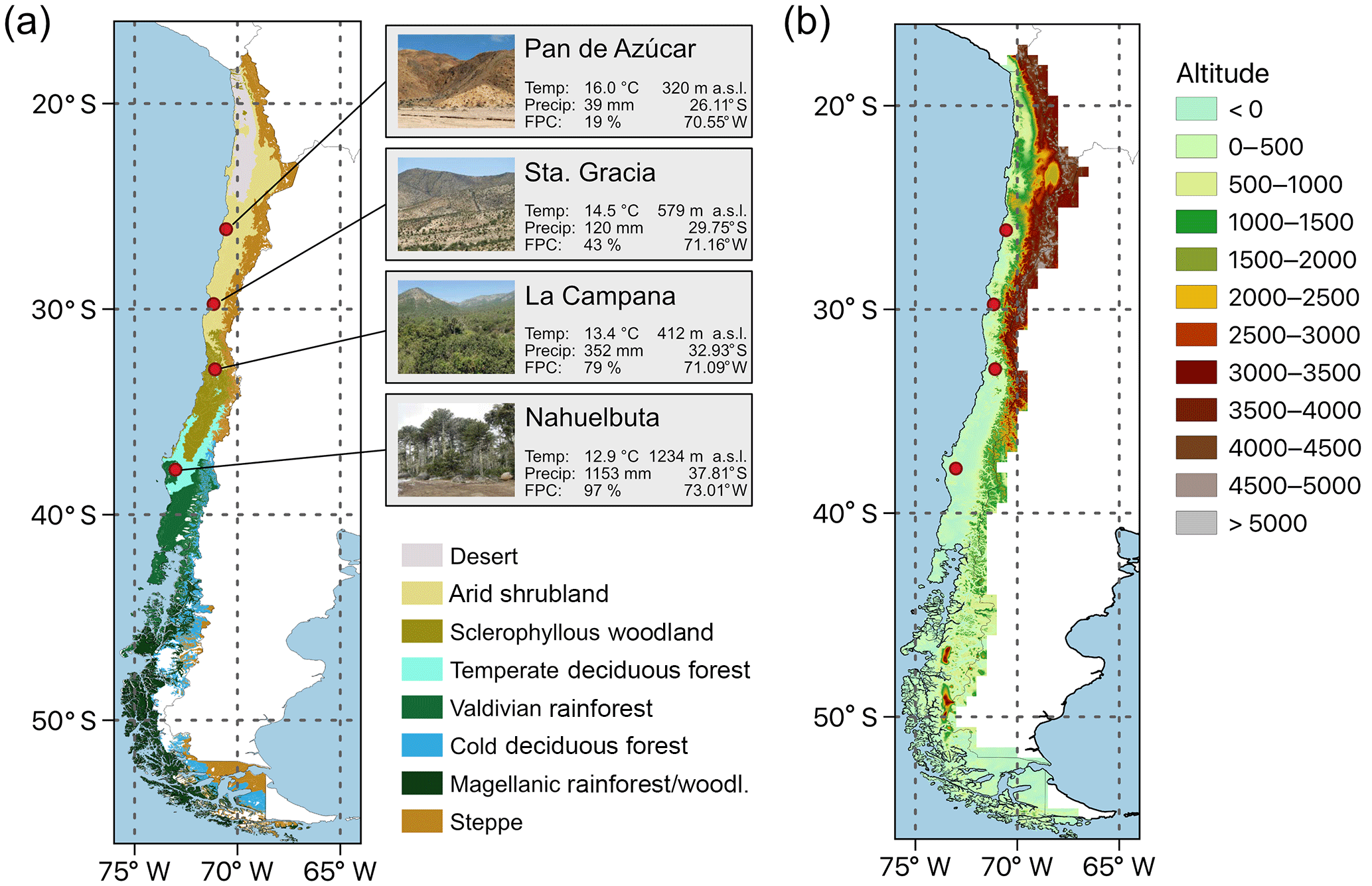
Figure 1(a) Distribution of major vegetation zones in Chile the and location of the four EarthShape SPP focus sites: Pan de Azúcar, Sta. Gracia, La Campana, and Nahuelbuta (“Temp” represents average annual temperature, “Precip” represents average annual precipitation – data: ERA-Interim 1960–1989, and “FPC” represents foliage projected cover (MODIS VCF v6, total vegetation cover, 2001–2016 average, Dimiceli et al., 2015). Vegetation zones are based on Luebert and Pliscoff (2017). (b) Elevation of the model domain.
This study is part of the German EarthShape priority research program (https://www.earthshape.net, last access: 15 September 2018), which investigates how biota shapes Earth surface processes along the climatic gradient of the Coastal Cordillera of Chile. Here, we describe the climate data processing and vegetation modeling approach, and report results of simulations for the last 21 000 years. Specifically, we (a) develop a regionally adapted setup of LPJ-GUESS that also includes improvements in the sub-grid representation of vegetation (required for future coupling), (b) simulate potential natural vegetation (PNV) for Chile for present day (PD), MH, and LGM climate conditions, and (c) conduct transient simulations for four focus sites (Fig. 1a) at a monthly resolution spanning the full period from the LGM to the PD. Furthermore, we (d) investigat the effect of [CO2] and the use of different paleoclimate data for vegetation simulations of the LGM, and (e) explor the relationship between vegetation state, vegetation cover, and simulated surface runoff. A companion paper (part 2, Schmid et al., 2018) presents a sensitivity analysis of how transient climate and vegetation impact catchment denudation. This component is evaluated through the implementation of transient vegetation effects for hillslopes and rivers in a LEM. Although the approaches presented in these two companion papers are not fully coupled, the results of predicted vegetation cover change derived from our vegetation simulations provide the basis for the magnitudes of change in vegetation cover implemented in the companion paper. Together, these two papers provide a conceptual basis for understanding how transient climate and vegetation could impact catchment denudation. As a follow-up to these two studies we plan to couple the vegetation and LEMs.
Climate and vegetation are key controls of the surface processes that shape landscapes. This is due to the fact that precipitation enables the transport of sediment down-slope, while vegetation cover has the ability to protect hillslopes from erosion due to root cohesion, obstruction of overland flow, and protection from splash erosion. Vegetation characteristics (i.e., composition and cover, which vary substantially by life-form, rooting, and phenological strategies) are not constant in space and time and vary with climate, topography, and soils. Furthermore, environmental forcing such as temperature, precipitation, radiation, and [CO2] change over longer timescales and lead to different vegetation assemblages, potentially differing vegetation cover, and thus protection from erosion.
2.1 Climate of Chile
Chile's location bordering the Pacific Ocean, its vast meridional extent of 4345 km, and its steep topographic longitudinal profile (Fig. 1b) result in highly variable climatic conditions. The large-scale subsidence of air masses over the southeast Pacific Ocean and other regional factors (e.g., relative cold coastal ocean currents) yield extremely arid desert conditions in northern Chile with as little as 2–20 mm of annual precipitation (Garreaud and Aceituno, 2007). In the south, a 1000 km long narrow band of Mediterranean-type climate exists on the western side of the Andes (Armesto et al., 2007). According to a general bioclimatic classification by Luebert and Pliscoff (2017), the tropical/Mediterranean boundary is located from 23∘ S (coast) to 27–28∘ S (inland) and the Mediterranean/temperate boundary is located at 36∘ S (in both the Chilean Coastal and Andes mountain ranges) to 39∘ S (the “Central Depression”), while the temperate/boreal boundary is found from 50.5 to 56∘ S. From a climatologic standpoint, the Mediterranean bioclimatic region has a warm temperate climate dominated by winter rain (the mean annual precipitation varies from 300 to 1500 mm from north to south, respectively) and hot, dry summers with dry periods varying from 7 months (north) to less than 4 months (south) in duration (Uribe et al, 2012). To the south, midlatitude westerly winds and orographic uplift by the coastal mountains and the Andes lead to an annual precipitation of up to 3000 and 5000 mm, respectively (Veblen et al., 1996). El Niño occurrences generally lead to above average precipitation rates in the austral winter and spring in the Mediterranean zone and reduced precipitation at 38–41∘ S in the following austral summer (Garreaud and Aceituno, 2007; Montecinos and Aceituno, 2003).
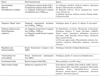
Table 1Major vegetation zones, associated plant functional types (PFT), and representative species (modified after Escobar Avaria, 2013; Luebert and Pliscoff, 2017; the letters a–e are given to help the reader identify the PFT and the representative species).
2.2 Vegetation of Chile
Considering the ecological divisions of South America (Young et al., 2007), Chile is represented by three noticeable areas: the Peruvian–Chilean desert, Mediterranean Chile, and the moist Pacific temperate area. These areas reflect the main floristic characteristics and vegetation types of the country; moreover, the distribution of vegetation within these areas is constrained by thermal and hydrological climatic factors that vary according to latitude and longitude (see Table 1 for an outline of the characteristic species, the biome classification, and modeled vegetation types). In the north, longitudinal variations in climate are the result of geomorphological and ombroclimatic changes. Between 17 and 28∘ S, the coastal zone is exposed to the influence of fog and orographic precipitation, allowing vegetation such as columnar cacti (Eulychnia genera) and a diverse group of shrubs (e.g., Nolana, Heliotropium, Euphorbia, Tetragonia) and succulents (e.g., Deuterocohnia, Tillandsia, Puya, Neoporteria) to develop (Luebert and Pliscoff, 2017). To the west, and between the Chilean Coastal and the Andes mountain ranges, a hyper-arid desert zone exists, which is characterized by the absence of rainfall or coastal-fog water inputs; therefore, no vascular plants are usually found in this area. However, with punctual water inputs due to local substrate conditions, such as the presence of a water table, some halophytic shrubs (e.g., Prosopis sp.) can develop (Luebert and Pliscoff, 2017). Vegetation in the Andes mountain range is constrained by altitude due to the decrease in temperature and the increase in precipitation. The major development regarding vegetation is observed at intermediate altitudes where shrubs tend to dominate (Luebert and Pliscoff, 2017).
Vegetation increases to the south with increasing winter precipitation (Rundel et al., 2007), allowing Mediterranean-type shrubland and woodland ecosystems to develop. In these ecosystems various plant species, commonly denominated sclerophyllous plants, have small, rigid, xeromorphic leaves adapted to hot, dry summers and wet, cool winters (Young et al., 2007). Sclerophyllous woodlands and forests extend from 30–31 to 37.5–38∘ S (Fig. 1a) and range from xeric thorn savanna elements to dense herbaceous cover in the Central Depression, whilst evergreen sclerophyllous trees and tall shrubs are found at higher elevations in which mesic conditions predominate. In these ecosystems, slope aspect can modify local moisture conditions, affecting the structure and composition of vegetation (Luebert and Pliscoff, 2017). To the south, these vegetation types transition into temperate deciduous Nothofagus forests (Maule or Nothofagus parklands. The dominant species in these areas being Nothofagus obliqua, N. glauca, and N. alessandrii) at the Coastal Cordillera and lower Andes ranges, before forming a broader vegetation zone (Donoso, 1982; Villagrán, 1995). The deciduous Nothofagus forests then grade into mixed deciduous–evergreen Nothofagus forests at 36∘ S (Young et al., 2007). With increasingly hydric conditions evergreen broad-leafed species begin to dominate forest stands at approximately 40∘ S and form the Valdivian rainforest (the northernmost rainforest type, ranging from 37∘45′ to 43∘20′ S) with high biomass and arboreal biodiversity and evergreen, deciduous, and needleleaf species (Veblen, 2007). Further south, the less diverse North Patagonian rainforest is mainly dominated by Nothofagus betuloides (Veblen, 2007) and transitions into the Magellanic rainforest at approx. 47.5∘ S and Magellanic moorland with waterlogged soils and a poor nutrition status at the coast (Arroyo et al., 2005). Cold deciduous forests stretch from 35 to 55∘ S along the Andes covering cooler and dryer sites as compared to the coastal rainforests. These forests occur at altitudes of approx. 1300 m and gradually descend to sea level in Tierra del Fuego (Pollmann, 2005). In Tierra del Fuego and east of the low Andes in southern Patagonia a gramineous steppe exists (Moreira-Muñoz, 2011), and a high-Andean steppe also extends north at higher altitudes.
3.1 Vegetation model
The Lund-Potsdam-Jena General Ecosystem Simulator (LPJ-GUESS; Smith et al., 2001, 2014) is a state-of-the-art dynamic vegetation model that also simulates detailed stand dynamics using a gap-model approach (Bugmann, 2001; Hickler et al., 2004). The model is developed by an international community of scientists and has been used in more than 200 peer-reviewed international publications, including model evaluations against a large variety of benchmarks such as vegetation type distribution, vegetation structure and productivity, as well as carbon and water cycling at regional to global scales (https://www.nateko.lu.se/lpj-guess, last access: 15 September 2018). Vegetation development and functioning is based on the explicit simulation of photosynthesis rates, stomatal conductance, phenology, allometric calculations, and carbon and nutrient allocation. The model simulates the growth and competition of different plant functional types (PFT, see Bonan et al., 2002) based on their competition for space, water, nutrients, and light. Population dynamics are then simulated as stochastic processes that are influenced by current resource status, life history, and demography for each PFT. To enable a representative description of average site conditions within a landscape each grid cell is simulated as a number of replicate patches in order to allow different (stochastic) disturbance histories and development (successional) stages (see Hickler et al., 2004; Wramneby et al., 2008). Fire occurrence is determined by the model using temperature, fuel load, and soil moisture levels (Thonicke et al., 2001). Soil hydrology in LPJ-GUESS is represented by a simple two-layer bucket model with percolation between layers and deep drainage (see Gerten et al., 2004).
Vegetated surface area and runoff are affected by a range of model parameters in LPJ-GUESS. In “cohort” mode, an average individual from each PFT with a given age and development status is used to characterize vegetation state. Depending on PFT-specific parameters (i.e., maximum crown area, sapling density, allometric properties, leaf-to-sapwood area), age, and competition for light, water, space, nutrients, and demographic processes (establishment and mortality) individual cohorts can develop different states.
Using Eq. (1), we approximate the fraction A of the land surface covered by vegetation using the foliar projected cover (FPC) – the vertical projection of leaf area onto the ground (see Wramneby et al., 2010). In LPJ-GUESS the FPC is derived from daily leaf area index (LAI, the leaf area to ground area ratio, m2 m−2) summed for all simulated PFTs (n refers to the number of PFTs) using the Lambert–Beer extinction law (originally proposed by Monsi and Saeki in 1953 for the estimation of light extinction in plant canopies, see translation in Monsi and Saeki, 2005; Prentice et al., 1993):
Thus, depending on the composition of PFTs and the disturbance regime, varying levels of ground cover can be simulated that not only reflect the environmental conditions but also vegetation diversity and development.
In addition, the hydrological cycle is also affected by PFT-specific interception and transpiration rates that are a function of PFT-specific parameters and the development stage. Thus, vegetation modulates infiltration via interception (that is a function of vegetation cover) and runoff (via plant uptake and transpiration of water) under the given environmental constraints. In LPJ-GUESS water enters the top soil layer as precipitation until this layer is fully saturated (excess water is lost as surface runoff, and evaporation removes water from a 20 cm sub-horizon of the top layer). During precipitation days, water can percolate from the top to the lower layer until the lower layer is saturated (excess water is lost as drainage). In addition, water from the lower layer can drain as baseflow with a fixed drainage rate (Gerten et al., 2004; Seiler et al., 2015). The model does not consider lateral water movement between grid cells nor does it take routing in a stream network into account (in this study we report the surface runoff component only).
3.2 Landform classification
To bridge the gap in spatial resolution between LPJ-GUESS (typical spatial resolution of ) and the LEM Landlab (Hobley et al., 2017; Schmid et al., 2018, typical spatial resolution ∼100 m) and facilitate the future coupling of these models, we introduced the concept of landform disaggregation of grid cell conditions to smaller sub-pixel entities (Figs. 2, B1). The advantages of introducing sub-pixel entities as opposed to simply performing higher-resolution simulations are twofold. Firstly, higher-resolution simulations require climate forcing data of the desired output resolution that are not available for the intended simulation periods or region (and are not generally available for past time periods). Secondly, using sub-pixel entities incurs smaller additional computation costs than higher-resolution simulations.
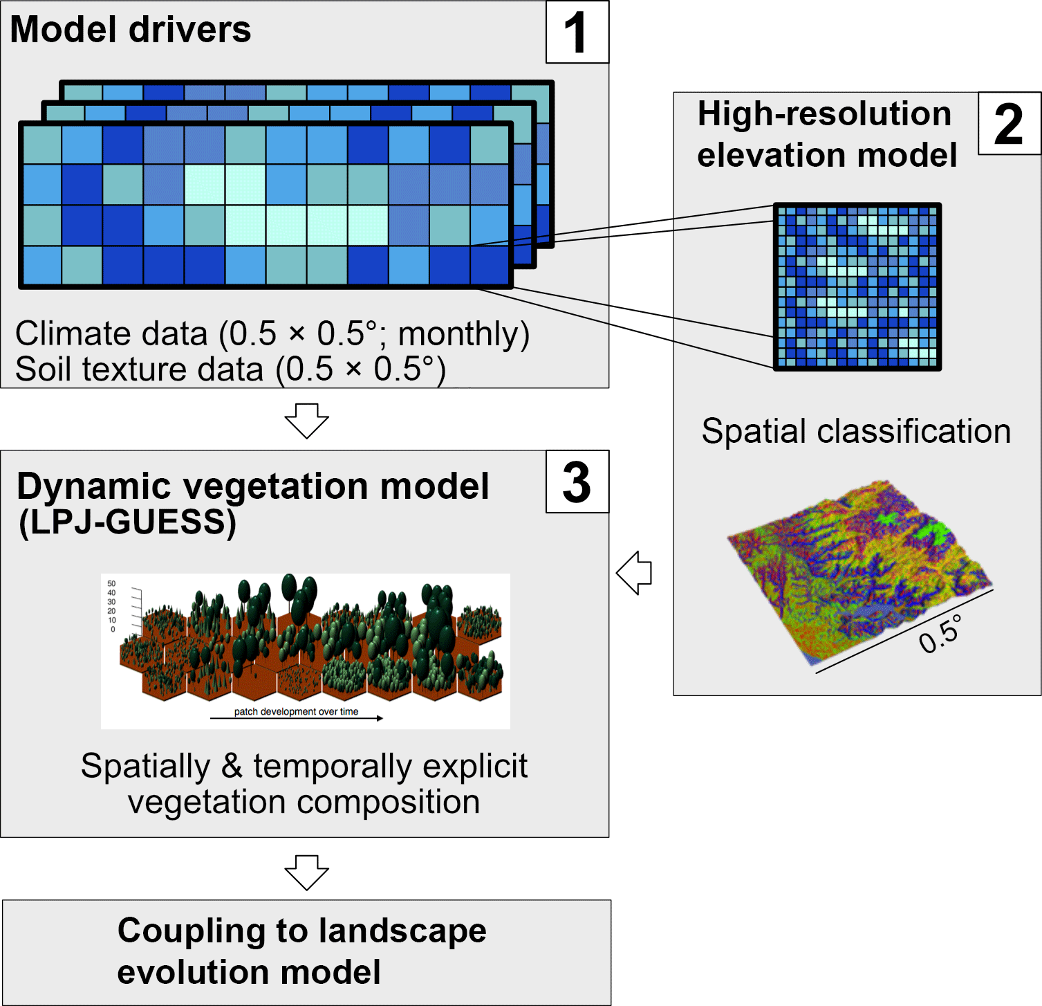
Figure 2Schematic procedure of simulations. Coarse resolution model driving data (1) is disaggregated using a high-resolution elevation model and topographic landform classification (2), and the ecosystem model LPJ-GUESS then simulates vegetation state and dynamics using the landform classification to simulated topographic-adjusted patch composition (3). Vegetation cover and surface runoff results can then be passed on to a coupled landscape evolution model (LEM) (not implemented in this study, see Schmid et al. (2018) for a description of the LEM).
Sub-pixel entities, hereafter termed “landforms”, were derived for each grid cell using SRTM1-based elevation models (Kobrick and Crippen, 2017). Pixels from the elevation model (30 m spatial resolution) were classified based on their elevation (200 m bands) and their association with topographic features (ridges, mid-slope positions, valleys, and plains – based on slope and aspect), and similar pixels were grouped to form the landforms. The elevation of the landforms was used to modify the temperature at a given landform. Using the elevation difference between the average elevation of a landform as derived from the high-resolution elevation model and the reference elevation obtained from the grid, a temperature delta was calculated using the lapse rate from the International Standard Atmosphere model of −6.5 ∘C km−1 (e.g., Vaughan, 2015). However, it should be noted that this lapse rate is a global average rate that can substantially differ from local conditions and over multiple timescales (ranging from sub-daily to climatological), as it is controlled by various atmospheric thermodynamics and dynamics (i.e., radiative conditions, moisture content, large-scale circulation conditions). While a higher lapse rate would potentially be a better approximation for drier sites (e.g., Pan de Azúcar), this might not be the case for other sites or past time periods with different atmospheric conditions. Furthermore, the lack of defining environmental data and a mismatch of scales prohibits the use of more specific regional lapse rates in our simulations.
The slope and aspect were utilized to adjust the incoming radiation received by the landform (see Appendix B). The general topographic features were used to modify the depth of the lower soil layer (deeper soils in valleys and on plains, shallow soils on ridges) and to identify areas (valleys and plains) with a newly implemented time-buffered deep-water storage pool that is only accessible by tree PFTs. The classification resulted in 2 to 56 (the mean was 17) landforms for each grid cell depending on the topographic complexity.
In the proposed future coupled model, we envisage that the landform classification will be performed using elevation information from the LEM. The resulting per-landform (but non-spatially explicit) vegetation simulation results will be matched back to spatially explicit grid cells in the LEM, which will allow us to bridge the scale gap between the two models.
In the simulations presented here, all classified landforms with an area > 1 % of the total land area in a grid cell were simulated using 15 replicate patches each, and simulation results were aggregated by area-weighting the results to the grid cell level. For a summary of the implementation details see Fig. B1.
3.3 Parameterization of plant functional types and biome classification
In a previous study Escobar Avaria (2013) implemented the first regional simulation for Chilean ecosystems (also using LPJ-GUESS) for present day (PD) climate conditions using a region-specific parameterization, which the presented study adapts and builds upon. Eleven PFTs – three shrub types, seven tree types, and one herbaceous type – were defined in order to describe the major vegetation communities of Chile (Table C1). The definition of these PFTs are generally based on the proposed macro-units of Chilean vegetation (Luebert and Pliscoff, 2017) and follow the concept of representative/or dominant species for describing a physiognomic unit. Apart from growth habit and associated traits, PFTs were designed to differentiate between leaf morphology and strategy, shade-tolerant and shade-intolerant varieties, their adaption to water access (mesic, xeric type), and root distribution. An overview of major eco-zones, associated PFTs, and representative species is given in Table 1.
Using a biomization approach (see Prentice and Guiot, 1996 for the general concept), we classified the simulated PFTs into discrete vegetation types (referred to as biomes throughout the paper; see Fig. C1 for details of the classification procedure). Based on LAI thresholds and the ratio of certain key PFTs or PFT groups (i.e., boreal tree PFTs, xeric PFTs) to their peers, a cascading decision tree was implemented that led to 11 biomes resembling the general vegetation zones of Chile (Fig. 1a), but also included additional biome classes to capture the finer nuances of transitions between semi-arid and mesic vegetation communities and open woodlands. To keep the number of vegetation types reasonable we designed multiple decision paths for biomes that exist as dense forest ecosystems but also transition into lower canopy woodlands or transition into more open woodlands (i.e., Magellanic forest, cold deciduous forest; see Fig. C1). The classification was conducted at the landform level after the simulated 15 patches were averaged, and the grid cell classification was derived from picking the area-dominant class of the landforms of a grid cell.
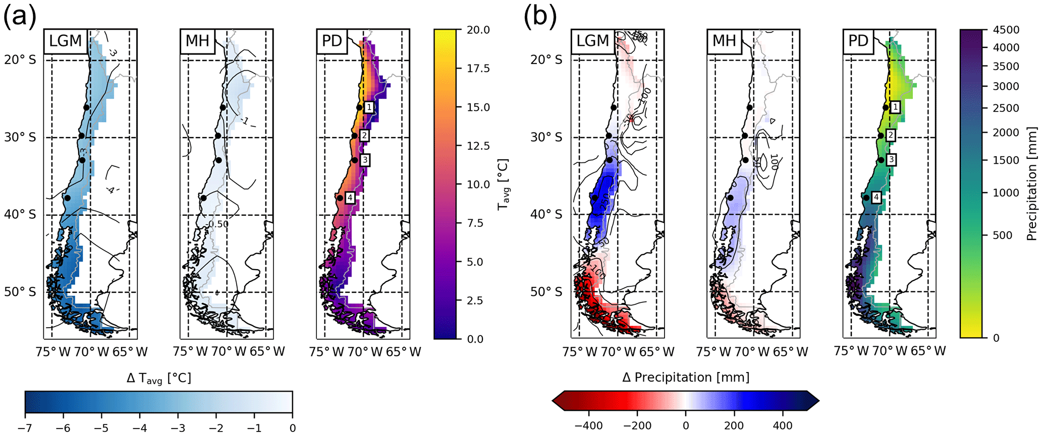
Figure 3(a) Average annual temperature and (b) precipitation derived from the downscaled and bias-corrected TraCE-21ka transient paleoclimate data (Liu et al., 2009) for the Last Glacial Maximum (LGM), mid-Holocene (MH), and present day (PD) time slices (data is the average of 30 year monthly data; 1 represents Pan de Azúcar, 2 represents Sta. Gracia, 3 represents La Campana, and 4 represents Nahuelbuta).
3.4 Environmental driving data and modeling protocol
The climate forcing data for LPJ-GUESS is derived from TraCE-21ka (Liu et al., 2009), which is a transient coupled atmosphere–ocean simulation from LGM to PD using the Community Climate System Model version 3 (CCSM3; Collins et al., 2006). In this study we present time-slice simulations for the LGM, MH, and PD (1960–1989), using perpetual climate forcing data from 30-year monthly climatologies (Fig. 3). In addition, we show results from a transient model simulation that utilizes the full time-series data from the LGM to PD. All simulations were preceded by a 500-year spin-up period with de-trended climate data until vegetation and soils reached steady state. For time-slice simulations the last 30 years of the simulation were used.
Monthly temperature, precipitation, and downward shortwave radiation from the TraCE-21ka dataset (resolution T31; ) were downscaled to a spatial resolution and bias-corrected using a monthly climatology from the ERA-Interim reanalysis (Dee et al., 2011, years 1979–2014). We used an additive bias correction for the temperature and multiplicative corrections for the precipitation and shortwave radiation (see Hempel et al., 2013; this technique was also used in, e.g., O'ishi and Abe-Ouchi, 2011). The multiplicative corrections for the precipitation and radiation are necessary because these fields can not have negative values. The resulting bias-corrected anomalies were subsequently downscaled to the ERA-Interim grid using a bilinear interpolation technique. The number of rain days within each month (used by LPJ-GUESS to distribute monthly precipitation totals to daily time steps internally) was derived from the monthly mean precipitation in the TraCE-21ka data and the day-to-day precipitation variability from ERA-Interim (see Appendix A). The [CO2] for each simulation year was obtained from Monnin et al. (2001) and Meinshausen et al. (2017). A comparison climate dataset for the LGM (referred to as ECHAM5 in this paper) was provided by Mutz et al. (2018). Soil texture data used for bare-ground initialization of the model was obtained from the ISRIC-WISE soil dataset (Batjes, 2012) and a default soil depth of 1.5 m (0.5 m topsoil, 1 m subsoil) was assumed.
We simulated vegetation dynamics using the process-based dynamic vegetation model LPJ-GUESS (Smith et al., 2001) version 3.1 (Smith et al., 2014) with the model additions outlined above. The model runs were carried out without nitrogen limitation, using the CENTURY carbon cycle model (see Smith et al., 2014). Patch destroying disturbance and establishment intervals were defined as 100 and 5 years, respectively, and fire dynamics were enabled. Further details of the PFT specific parameterizations are given in Table B1. The transient site-scale model runs were only conducted for the four focus sites of the EarthShape SPP due to (i) computing resource constraints, (ii) better comparability with other EarthShape SPP work (see Schmid et al., 2018), and (iii) better interpretability.
In this study we present data from two types of simulations. First, we show results for time-slice (LGM, MH, PD) simulations. Direct model results (simulated LAI of individual PFTs) are presented first (Sect. 4.1) and then aggregated to a biome representation for easier visualization and comparison (Sect. 4.2). Next, foliar projected cover and surface runoff are investigated (Sect. 4.3). Then, we present results from the transient LGM-to-PD site simulations (Sect. 4.4), and finally a sensitivity analysis of the effect of [CO2] levels under LGM climate conditions on vegetation composition and cover is carried out (Sect. 4.5).

Figure 4Spatial and altitudinal distribution of modeled plant functional types (PFT) for present-day climate conditions (LAI is the leaf area index – units m2 m−2; the altitudinal subplot represents zonal mean LAI; the red line represents the average elevation). PFTs are as follows: TeBEtm∕TeBEitm (temperate broad-leaved evergreen trees; t is shade-tolerant, it is shade-intolerant, m is mesic), TeBEitscl (temperate broad-leaved evergreen trees; scl is sclerophyllous), TeBSim/TeBSitm (temperate broad-leaved summergreen trees), TeEs (temperate evergreen shrubs; s is shrub), TeRs (temperate raingreen shrubs), TeNE (temperate needle-leaved evergreen trees), BBSitm (boreal broad-leaved summergreen trees), BBEitm: (boreal broad-leaved evergreen trees), BEs (boreal evergreen shrubs), C3G (herbaceous vegetation). The number 1 represents Pan de Azúcar, 2 represents Sta. Gracia, 3 represents La Campana, and 4 represents Nahuelbuta.
4.1 Distribution of simulated plant functional types
Vegetation communities (expressed as assemblages of PFTs in LPJ-GUESS) establish spatially depending on (a) environmental controls, (b) competition, and (c) stochastic events (i.e., fire incidents and mortality). An overview of the simulated vegetation distribution expressed as the simulated LAI for each PFT under PD climate conditions is given in Fig. 4 (for key PFT properties see Table C1; the PFT distribution maps for the MH and the LGM are given in the Supplement as Figs. S1 and S2 for completeness). Temperate broad-leaved evergreen trees (TeBEtm, TeBEitm; t represents shade-tolerant, it represents shade-intolerant, and m represents mesic) dominate the coastal and central areas from latitudes 40 to 46∘ S but also extend north into the Mediterranean zone. Further to the north, temperate broad-leaved summergreen PFTs (TeBStm, TeBSitm) occur, with the shade-tolerant type dominating a relative small area between 37 and 40∘ S. Northward, and in coastal areas, the sclerophyllous temperate evergreen PFT (TeBEitscl; scl represents sclerophyllous) starts to dominate, and with dryer conditions the total LAI (LAItot) is dominated by evergreen and raingreen shrubs (TeEs, TeRs; s represents shrub). South of 40∘ S, and in higher terrain as well as further north, boreal broad-leaved summergreen and evergreen tree PFTs (BBSitm, BBEitm) as well as boreal evergreen shrubs (BEs) establish. In the Andean ranges and (to a lesser extent as secondary components) in the lowlands and coastal ranges from 35 to 50∘ S, temperate needle-leaved evergreen trees (TeNE) are simulated. Herbaceous vegetation (C3G) dominates LAItot at high altitudes along the Andean ranges and is also a substantial contributor to the total LAI in the Mediterranean zone (30 to 38∘ S). Herbaceous vegetation also contributes to a lesser extent in most other regions, except for in the hyper-arid desert areas. LAItot is highest in the zone from 36 to 50∘ S. While LAI decreases substantially at sea level towards the Atacama Desert, higher values of the LAI are found further north at higher altitudes (see inset in Fig. 4).
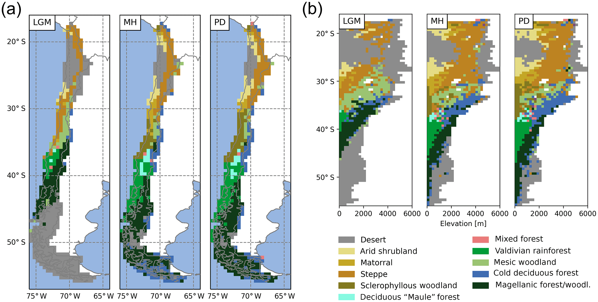
Figure 5(a) Spatial and (b) altitudinal distribution of biomes for Last Glacial Maximum (LGM), the mid-Holocene (MH), and the present day (PD) (for the biome classification decision tree see Fig. C1).
4.2 Distribution of simulated biomes at LGM, MH, and PD
The simulated biome distribution changes spatially (Fig. 5a), vertically (Fig. 5b), and over time. Under PD climate, the simulated Valdivian temperate rainforests extend from 38 to 46∘ S at the coast and transition into the Magellanic forests/woodlands, that are dominated by the boreal PFTs. A small zone of deciduous “Maule” forest occurs to the north of the Valdivian rainforest at meso-temperate climates. With even dryer and warmer conditions the sclerophyllous woodland type establishes and (as the fraction of trees and LAItot is reduced even further with increasing temperatures and even lower annual rainfall) eventually give way to shrub dominated matorral and finally the arid shrubland biome type. The cold deciduous forest type is classified for parts of Tierra del Fuego, and at higher elevations in the lower Andes in Patagonia. It also forms larger zones at altitude between 30 and 40∘ S. Mesic woodland occurs between 34 and 30∘ S at altitude (above the sclerophyllous woodland zone dominating the lowlands), and high-Andean steppe occurs between 18 and 30∘ S. A cold desert is present above the tree line in Patagonia and the highest Andean ranges, whereas hot desert (LAItot < 0.2) is simulated for areas from 20 to 26∘ S. The model was able to simulate the general distribution of the biomes of Chile for most regions (Figs. 1a, 5), although accuracy for the occurrence of deciduous PFTs was low (deciduous “Maule” forest and cold deciduous forest, also previously reported by Escobar Avaria, 2013).
Owing to the similarity in climatic conditions (Fig. 3), the distribution simulated for the MH does not differ substantially from the PD (Table 2). The northern border of sclerophyllous woodland shifts to approx. 34∘ S, giving way to a matorral zone. In addition, the cold deciduous forest biome covers larger areas in Patagonia at the expense of Magellanic woodland (+27.5 % and −9.1 %, respectively; Table 2). However, the spatial and vertical distribution of biomes for the LGM is markedly different (Fig. 5a, b). The substantially lower temperatures (Fig. 3) lead to an expansion of cold deserts up to 45∘ S (coastal areas) and 40∘ S (higher altitudes), respectively. The boreal PFT dominated Magellanic woodland biome is substantially reduced in extent (16.5 % in the LGM versus 32.6 % in the PD of simulated area, Table 2) and is shifted further north (40 to 45∘ S at the coast, 43 to 35∘ S at higher altitudes inland). The area covered by temperate rainforest is restricted to a small lowland area from 36 to 40∘ S, and the larger areas of cold deciduous forest at altitude are also substantially smaller (Fig. 5b; Table 2). Lowland steppe and mesic woodland biomes are simulated instead of matorral and sclerophyllous woodlands, and desert cover larger areas of the high-Andes to the north.
Table 2Areal extent of biomes in the simulation domain (units: percent of total area).
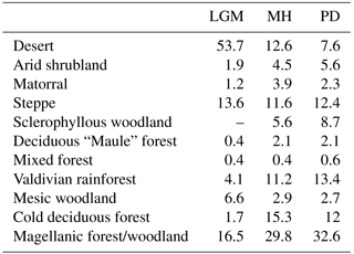
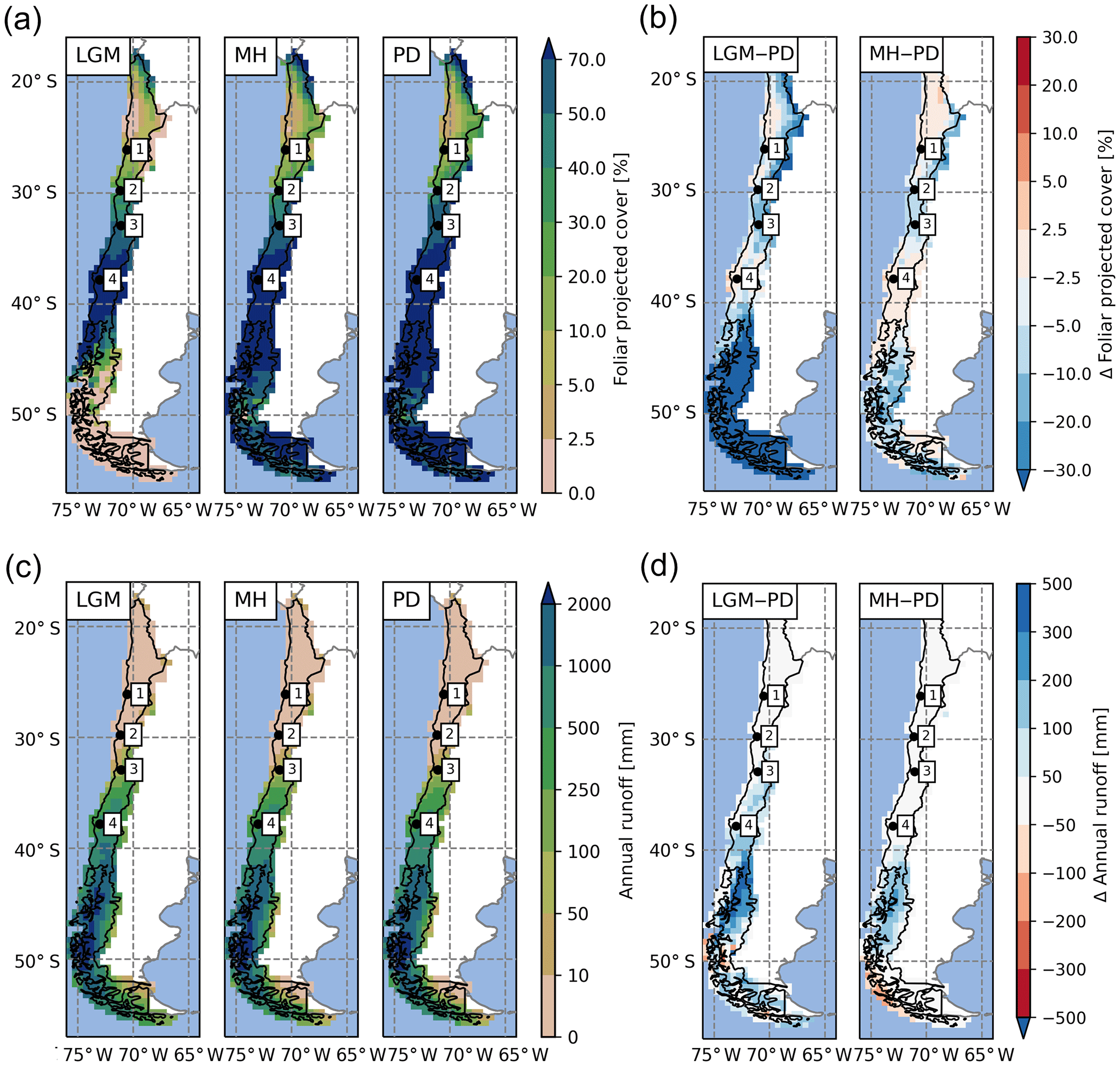
Figure 6Spatial distribution of (a) foliar projected cover and (c) surface runoff simulated for the Last Glacial Maximum (LGM), the mid-Holocene (MH), and the present day (PD). Difference plots of LGM versus PD (left) and MH versus PD (right) for foliar projected cover (b) and runoff (d), respectively (the number 1 represents Pan de Azúcar, 2 represents Sta. Gracia, 3 represents La Campana, and 4 represents Nahuelbuta).
4.3 Foliar projected cover and surface runoff
The percentage of ground covered, and thus shielded from strong denudation, and surface runoff (as a major driver of erosion rates) are both influenced by the composition and state of vegetation communities. Therefore, we evaluate the regional and temporal changes of these important variables as simulated by LPJ-GUESS for the LGM, MH, and PD time slices. The simulated LAI of PFTs can be aggregated and converted to foliar projected cover (see Eq. 1); thus, this allows us to estimate the surface covered by vegetation. However, it should be noted that this is only an approximation of true ground cover, as small-scale vegetation variations are not simulated in a location-specific fashion (spatial lumping effects are not considered for instance). Nevertheless, the implementation of a sub-grid landform scale was, in part, motivated to improve the models' prediction of smaller scale differences, as it should allow for the differentiation of different sub-grid conditions for the major landforms within one simulation cell (see Sect. 5.1 and Appendix B for further information). Low FPC clearly coincides with the distribution of hyper- to semi-arid biomes (Figs. 5a, 6a). Under PD climate conditions, average FPC for the semi-arid and Mediterranean biome types, including arid shrubland, matorral, and sclerophyllous woodland are 16 %, 35 %, and 66 % (Table 3), respectively, and cover increases southward with increases in annual precipitation rates (Fig. 3b). South of 35∘ S, FPC values > 70 % are simulated for most grid cells except for high-altitude locations, the glacier fields of North Patagonia, and parts of the Magellanic moorland at the coast (see also Table 3).
Table 3Average foliar projected cover (FPC) and annual surface runoff for simulated biomes for present day (PD) and relative change within these PD areas for the Last Glacial Maximum (Δ LGM, LGM-PD) and the mid-Holocene (Δ MH, MH–PD).
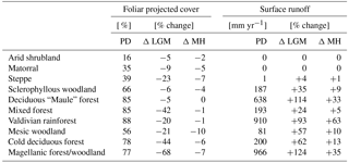
Simulated FPC was lower than satellite-based estimates by the MODIS Vegetation Continuous Fields product (Dimiceli et al., 2015), likely due to methodological differences in foliar projected cover and total satellite-observed vegetation cover, but the general patterns were represented (Fig. 7). The most distinct regional discrepancy can be observed in coastal areas between 30 to 36∘ S and the Andean highlands in the north of the model domain. For the entire model domain the mean average error (MAE) of the FPC was 11.9 %. The best agreements of 6.1 % and 6.3 % MAE were achieved for the arid shrubland and Valdivian rainforest biomes, while the discrepancies were greatest for mixed forest and cold deciduous forest biomes with 22.4 % and 22.1 % MAE, respectively (see Fig. 4a for biome locations; note that LPJ-GUESS often tends to underestimate the FPC of deciduous PFTs). A strong positive correlation between annual rainfall and FPC can be observed for all semi-arid, Mediterranean, and seasonally dry temperature eco-zones (Fig. 8a) and increases in annual rainfall lead to a strong rise of ground covered until 250–300 mm rainfall per year (arid shrubland: +14.5 %–16.3 % 100 mm−1; matorral: +12.9 %–16.5 % 100 mm−1; steppe: +13.5 %–17.8 % 100 mm−1; Fig. 8a). At these levels, Mediterranean and temperate woodland biomes start to dominate but increases in precipitation only raise FPC by +2.7 %–3.3 % 100 mm−1 and +5.4 %–6.4 % 100 mm−1, respectively (sclerophyllous woodland and mesic woodland).
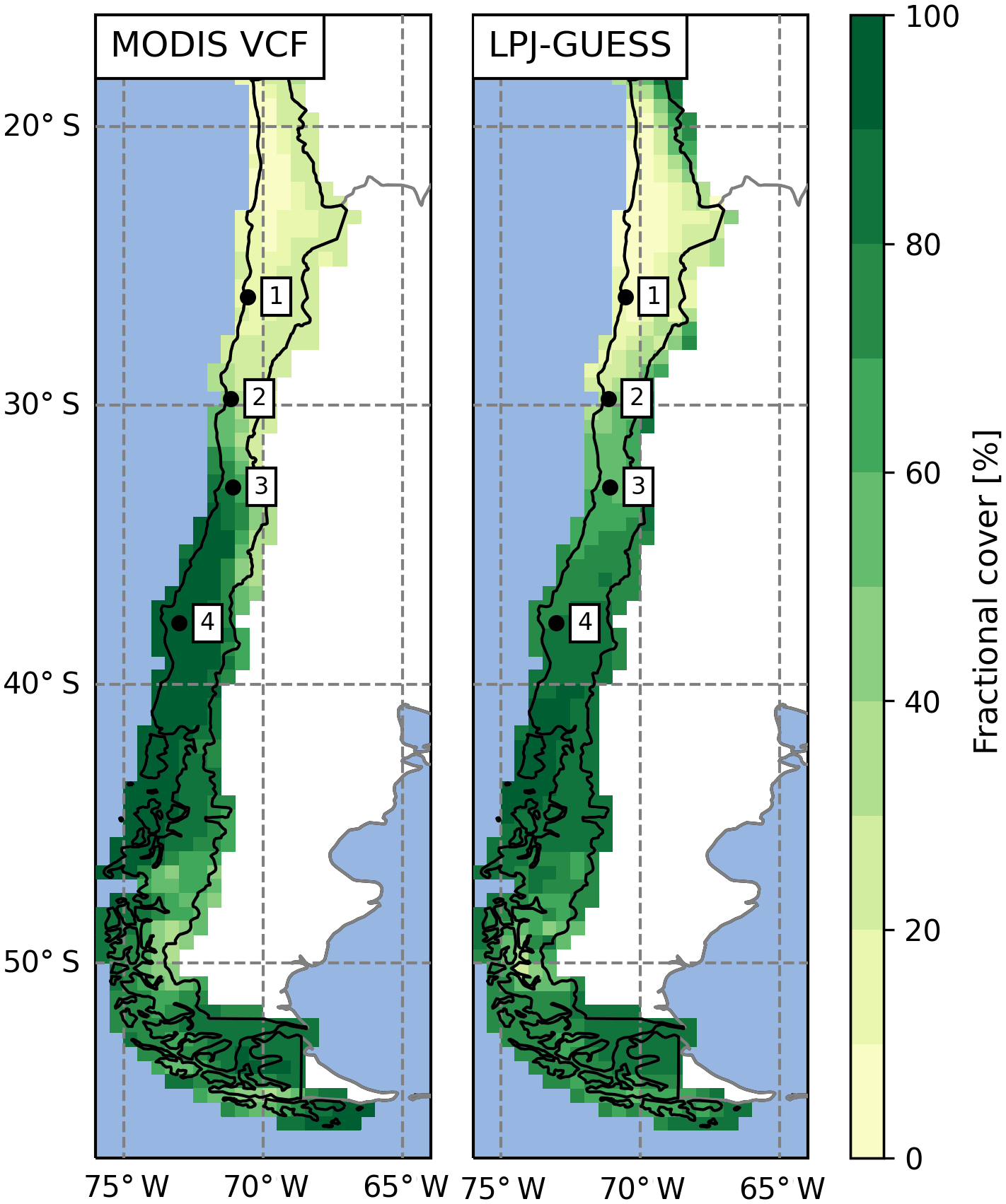
Figure 7Comparison of satellite-derived vegetation cover and simulated average foliar projected cover of potential natural vegetation for present day (data: MODIS MOD44B VCF v6, total vegetation, 2001–2016 average; Dimiceli et al., 2017; 1 represents Pan de Azúcar, 2 represents Sta. Gracia, 3 represents La Campana, 4 represents Nahuelbuta).
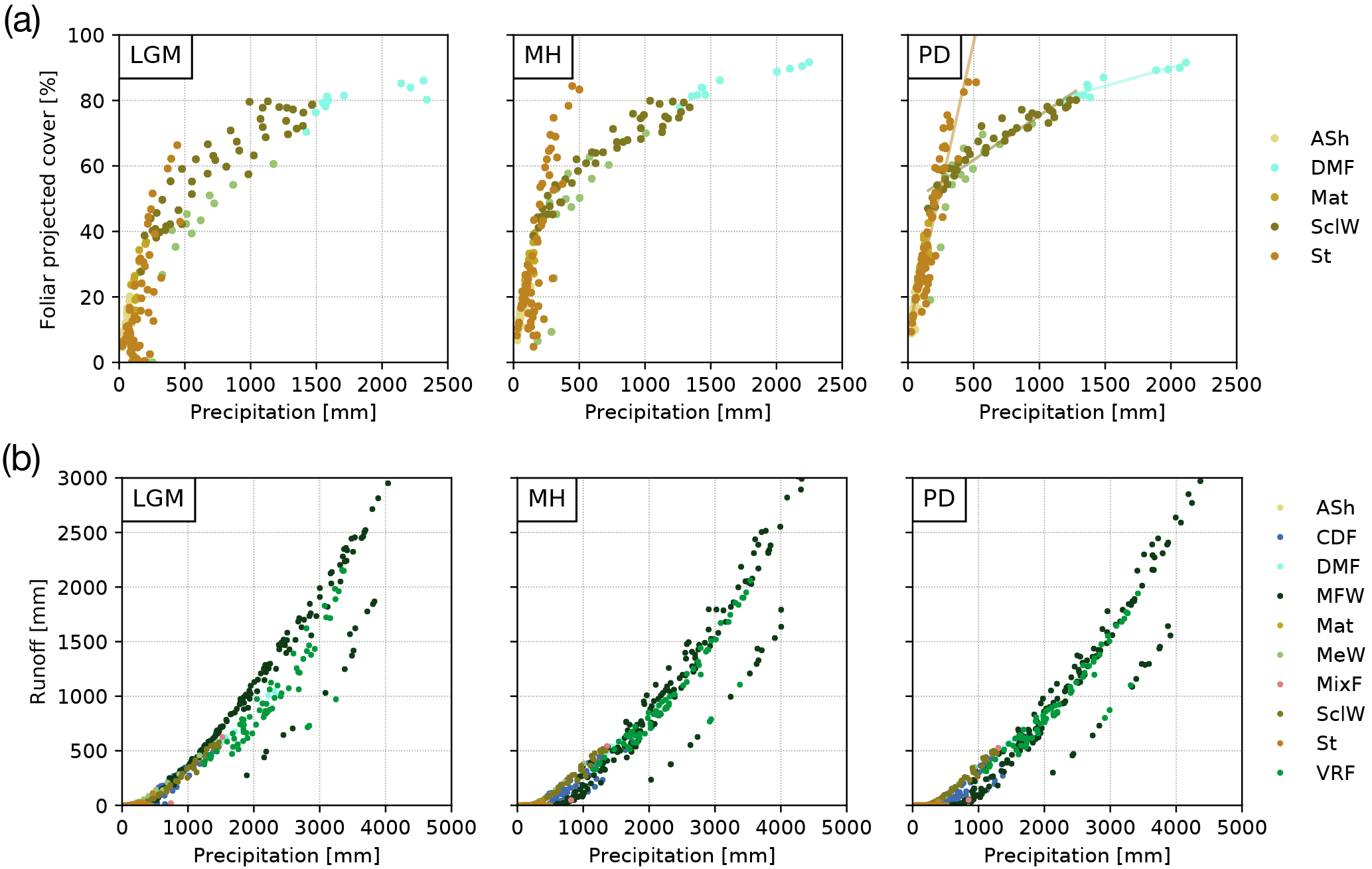
Figure 8(a) Foliar projected cover (FPC) and (b) surface runoff as a function of annual average rainfall for the Last Glacial Maximum (LGM), the mid-Holocene (MH), and present day (PD) (“ASh” is arid shrubland, “CDF” is cold deciduous forest, “DMF” is deciduous “Maule” forest, “MFW” is Magellanic forest/woodland, “Mat” is matorral, “MeW” is mesic woodland, “MixF” is mixed forest, “SclW” is sclerophyllous woodland, “St” is steppe, “VRF” is Valdivian rainforest; temperate and boreal forest biomes (CDF, MixF, VRF, MFW) excluded from subplot (a) as they are also strongly dependent on temperature.
A similar spatial pattern of FPC can be observed for the MH (Fig. 6a) and for the relationship to precipitation rates (Fig. 8a). No significant difference in FPC to PD conditions is apparent for the Atacama Desert or for most temperate forest areas from 36 to 42∘ S. FPC in high-Andes locations in the north and large parts of the Magellanic forest and cold deciduous forest biomes in the south is 10 %–20 % lower than under PD climate, whereas in the Mediterranean zone FPC is reduced by 5 %–10 % (Fig. 6b, Table 3). The reduction of MH FPC (47–54∘ S) coincides with a zone of lower temperature (> −0.5 ∘C, see Fig. 6b) and the areal extent of TeBE PFTs (Fig. S1). Lower [CO2] at MH compared to PD might also be the reason for a general reduction of biomass productivity; however regional differences of the other climate drivers (i.e., temperature, precipitation) do alter this general trend.
Due to lower temperatures and reduced precipitation rates at high altitudes and in the southern part of the country (Fig. 3), FPC during the LGM in these areas is simulated to be strongly reduced (< −30 %, cold desert conditions for large areas south of 46∘ S); however, the FPC was lower for all areas of Chile (Fig. 6b, Table 3) which was likely also the effect of substantially lower [CO2] (see Sect. 4.5 for a sensitivity analysis of the effect of the atmospheric CO2 concentration). While the general correlation of FPC to precipitation can also be observed for the LGM (Fig. 8a), the variability in vegetation cover in mesic and xeric woodlands appears to be larger – indicating the potential for greater variability in erosion rates within the same biome. The strongest correlations between annual precipitation and FPC were observed for sclerophyllous woodland (adjusted r2 values of 0.84, 0.91, and 0.9 for LGM, MD, and PD, respectively; p< 0.001).
Annual average runoff varies greatly from north to south (Fig. 6c) and coincides with annual precipitation (Figs. 3, 8b). For PD and MH climates, LPJ-GUESS simulated almost no surface runoff for arid and Mediterranean areas of Chile to approx. 32∘ S (see also Table 3). Thus, correlation between precipitation and runoff in the steppe and arid shrubland biomes was low (adjusted r2: 0.16–0.27, 0.12–0.37, 0.11–0.35 for LGM, MH, and PD, respectively; p < 0.01). For all other systems (excluding matorral and mixed forests), correlation coefficients were generally > 0.85 for all time slices; p < 0.001).
Runoff rates gradually increase southward and reach their peak (> 2000 mm yr−1) in areas of hyper-humid conditions along the Pacific coast. MH runoff rates are higher for areas of northern Patagonian and Magellanic rainforest (40–46∘ S), but lower for coastal areas of Magellanic moorlands (Fig. 6d). LGM runoff rates are higher for most areas (Table 3) and especially south of 34∘ S, with the strongest differences occurring from 40 to 46∘ S. However, we want to highlight that the low temporal variability of the TraCE-21ka precipitation data likely leads to a substantial underrepresentation of episodes of high hygric variability (see discussion).
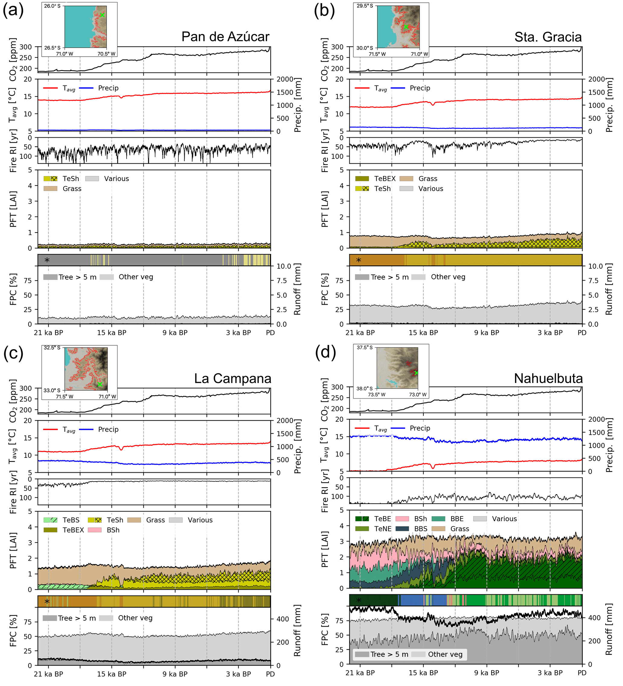
Figure 9Transient simulations for the (a) Pan de Azúcar, (b) Sta. Gracia, (c) La Campana, and (d) Nahuelbuta sites. The insets show the location within the simulated grid cell and the area and location covered by the landform plotted in this figure (results given in other figures are an area-weighted aggregation of individual landform simulation results). Panels 1–3 (from top to bottom): “Tavg” is annual average temperature, “Precip” is annual precipitation, “Fire RI” is fire return interval. Panel 4: “PFT” is plant function type; (grouped) PFT abbreviations: “TeSh” is temperate shrubs, “Grass” is herbaceous vegetation, “TeBEX” is sclerophyllous temperate broad-leaved evergreen trees, “TeBS” is temperate broad-leaved summergreen trees (hashed represents shade-intolerant), “BSh” is boreal evergreen shrubs, “TeBE” is temperate broad-leaved evergreen trees, “TeNE” is temperate needle-leaved evergreen trees, “BBS” is boreal broad-leaved summergreen trees, “BBE” is boreal evergreen trees, “Various” refers to other PFTs (LAI <0̇.05); plain represents shade-intolerant, hatched represents shade-tolerant, cross-hatched represents raingreen. Panel 5: “FPC” is foliar projected cover; trees and shrubs > 5 m are denoted using dark gray, herbaceous vegetation and small trees and shrubs are denoted using light gray. “Runoff” is simulated surface runoff; * Biomization: for a legend on the applied classification see Figs. C1 and 4 for a color-coded legend. All data smoothed using 100-year averaging.
4.4 Transient changes of simulated vegetation from LGM to present
In this section we present transient simulation results for grid cells that contain the EarthShape focus sites (Fig. 9). The results are given for a single landform of the simulated grid cells in order to preserve successional transitions between PFTs that might otherwise be lost through averaging. The field site location and the represented area of the chosen landform within the grid cell are marked in the insets of Fig. 9a–d. The diversity of simulated vegetation cover for all landforms of the four EarthShape focus sites is illustrated in Fig. B2. The area-averaged mean of landform enabled LPJ-GUESS simulations closely matches the default model results at the Sta. Gracia and La Campana sites, but FPC at the Pan de Azúcar and Nahuelbuta sites is approx. 3 % greater than the default simulation result (Fig. B2a). However, results from all four sites show that the inter-landform variability of FPC varies by 10 %, 15 %, 25 %, and 18 % for the Pan de Azúcar, Sta. Gracia, La Campana, and Nahuelbuta sites, respectively.
Temperatures and [CO2] start to increase at 18 000 BP and a marked pullback in temperatures during the Antarctic cold reversal (∼14 500 BP) is present in the TraCE-21ka data for all four sites (Fig. 9a–d). Annual precipitation at the Pan de Azúcar site (21.11∘ S 70.55∘ W, 320 m a.s.l.) is extremely low (38–40 mm, hyper-arid) for the entire simulation period (Fig. 9a). The annual average temperature for the landform presented increases from 13.9 ∘C (LGM) to 16.8 ∘C (PD). As a result of these arid conditions only evergreen and raingreen shrubs and herbaceous vegetation can establish, and LAI, and consequently FPC, remains very low (LAItot < 0.3). For most episodes of the simulation this location is classified as desert according to the implemented biomization scheme, with only two periods switching to another state (arid shrubland, LAItot > 0.2) from approx. 17 000 to 15 000 BP, and more permanently, the late Holocene. Fire return intervals (expressed as the number of years between fire incidents) fluctuate greatly as fuel production is substantially limited by low vegetation growth. No surface runoff is simulated and FPC ranges from 8 % (LGM) to 13 % (PD).
Climatic conditions for the Sta. Gracia site (29.75∘ S 71.16∘ W, 579 m a.s.l.) show a similar temporal progression from the LGM to PD, but average temperatures are lower and range from 11.9 ∘C (LGM) to 14.9 ∘C (PD) (Fig. 9b). Annual precipitation does not change substantially from the LGM to PD (152 versus 122 mm). Vegetation from the LGM to approx. 18 000 BP is dominated by herbaceous vegetation, but (raingreen) shrubs increase with rising temperatures, leading to a biome shift from steppe to matorral. Fire return intervals decrease with increased (arboreal) litter production due to the encroachment of shrubs but FPC only increases by 7 % from 33 % (LGM) to 40 % (PD). Simulated surface runoff is insignificant for most simulation years.
Temperatures at the La Campana site (32.93∘ S 71.09∘ W, 412 m a.s.l.) increase from 11.0 ∘C (LGM) to 14.0 ∘C (PD), but annual precipitation amounts decrease from 446 mm (LGM) to approx. 320 mm before slightly increasing again to 355 mm at PD. The simulated LGM vegetation for the La Campana site is dominated by herbaceous plants and small fractions of temperate evergreen deciduous trees mixed with small fractions of boreal shrubs which leads to a steppe biome classification with short episodes of mesic woodlands (Fig. 9c). With the decrease of annual precipitation and increasing temperatures (approx. 17 500 BP) sclerophyllous woodlands displace the deciduous trees and evergreen and raingreen shrubs start to appear. The fire-return intervals shorten in this phase and reach values of less than 15 years for the remainder of the simulation. Raingreen shrubs expand at approx. 12 000 BP and push back on herbaceous vegetation and, in part, evergreen shrubs. The LAI of sclerophyllous broad-leaved evergreen trees and shrubs further increases during the last 5000 simulation years, which leads to a shift in our biome classification from matorral (LAItot > 0.5) to sclerophyllous woodland (LAIwoody > 1). Despite pronounced changes in vegetation composition, FPC only increases from approx. 51 % (LGM) to 59 % (PD), which translates to a relative stable vegetation cover for these regions over time; thus, there is likely only a low impact of biome shifts on erosive processes.
Climatic conditions at the Nahuelbuta site (37.81∘ S 73.01∘ W, 1234 m a.s.l.) are markedly different to the three previously mentioned sites, as this location receives substantially higher annual precipitation throughout the time series (> 1200 mm) and average temperatures at this latitude and elevation are substantially lower (5.1 ∘C for LGM and 8.6 ∘C for PD, Fig. 9d). However, it can be seen that the landform is only representative of a small fraction of the grid cell as it is located on mountainous terrain, whereas most areas in the cell are covered by coastal lowlands with higher annual temperatures; thus, the site simulation results presented here differ from the total grid cell results presented in previous sections (see marked landform cover in inset; Figs. 9d and B2a, b). LPJ-GUESS simulates a diverse composition of PFTs and a transition from boreal, Magellanic woodland conditions at the LGM, to a period of cold deciduous forest (17 500–12 000 BP), followed by 12 000 years of Valdivian rainforest and mesic woodland alternations. During the LGM, boreal broad-leaved evergreen, deciduous tree, and shrub PFTs dominate and form a forest. Annual precipitation (> 1300 mm) and surface runoff (> 440 mm) is high during this period. With rising temperatures, the boreal shrubs and evergreen tree PFTs are displaced by temperate needle-leaved evergreen trees (TeNE) and increases in herbaceous vegetation. Temperate evergreen PFTs establish approx. 17 000 BP and, after another retreat at approx. 14 500 BP (coinciding with the Antarctic cold reversal), start to dominate the forest at this location. Fire frequency is low for the first 4000 simulation years and only rises to approx. 1 fire in 100 years afterwards. FPC remains at constantly high values (> 75 %) indicating a largely closed forest for the entire simulation period and thus low dynamics of erosive processes due to constant high vegetation cover in this area.
4.5 Sensitivity of foliar projected cover to [CO2]
The effectiveness of photosynthesis, and thus the plants ability to build up biomass, has a large dependence on [CO2] (Farquhar et al., 1980; Hickler et al., 2015). Increases in vegetation biomass (expressed in LAI) were observed in our simulations but coincide with a simultaneous rise in temperatures and [CO2] (Fig. 9b–d). To assess the direct effect of changes in [CO2], we conducted a sensitivity simulation under LGM climate conditions. We compared the default LGM simulations (TraCE-21ka, [CO2] ppm) with a preindustrial [CO2] level of 280 ppm (Fig. 10). This change led to an expansion of vegetated areas (high-Andean steppe), an increase of forest biomes at the expense of herbaceous vegetation (i.e., northward expansion of mesic woodland, cold deciduous forests, and Valdivian rainforest), and the establishment of small pockets of sclerophyllous woodland (Fig. 10a). In all vegetated areas FPC increased with higher [CO2], most notably between 30 and 40∘ S (+5–10 % FPC).
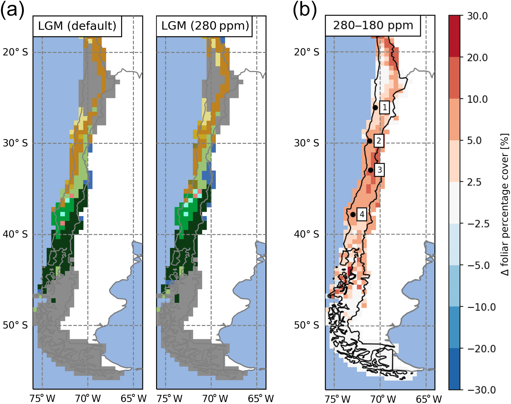
Figure 10(a) Effect of atmospheric CO2, represented as [CO2], concentrations on the simulated distribution of biomes for the Last Glacial Maximum (LGM) time-slice simulations (left panel: default LGM setup of this study with [CO2] =180 ppm; right panel: control run with preindustrial [CO2] =280 ppm). (b) Difference plot of resulting foliar projected cover (280–180 ppm). The number 1 represents Pan de Azúcar, 2 represents Sta. Gracia, 3 represents La Campana, and 4 represents Nahuelbuta.
The aim of this study was to demonstrate that a dynamic vegetation model with suitable modifications can simulate the state and transient changes of vegetation structure and composition at a temporal and spatial resolution that is suitable for coupling with LEMs which operate at higher spatial resolutions. To bridge the spatial scales and retain a high computational efficiency, we introduced sub-grid cell landform types in the DGVM LPJ-GUESS. Using this novel approach we are able to better reproduce observed spatial heterogeneity with existing DVMs. Furthermore, a regional parameterization of Chilean vegetation allowed us to simulated the present-day vegetation of Chile (Figs. 1a, 4, 5, 7; see also details in Sect. 5.1 below). In the PD simulations we found the largest regional discrepancy of observed and simulated vegetation cover to occur in coastal areas between 30 to 36∘ S, which might be attributed to the lack of fog precipitation in our model. Fog precipitation is strongly dependent on the distance to the coast, local topography, wind fields, and stratification of the troposphere (Lehnert et al., 2018) and can potentially contribute significant amounts of precipitation (Garreaud et al., 2008). However, a model representation of fog in LPJ-GUESS is difficult due to the scale mismatch and a lack of required input variables to determine the occurrence. Furthermore, precipitation amounts in the model drivers might be too low as the coarse spatial resolution of the original input data leads to an underrepresentation of orographic precipitation effects (i.e., Leung and Ghan, 1998). We also want to note that the MODIS VCF product was found to overestimate cover in sparsely vegetated areas (Sexton et al., 2013) and thus should rather be treated as a general guideline. Furthermore, LPJ-GUESS was applied to simulate the PNV, whereas MODIS VCF observes actual vegetation that includes anthropogenic land use (agricultural fields, degradation due to grazing, etc.).
Substantial changes in fire frequencies were observed in the transition simulations (Fig. 9b, c). LPJ-GUESS simulated these dynamics by considering available fuel which, in turn, is a function of present PFT composition and litter production. These rapid removals of vegetation cover have the potential to expose bare soil to erosion processes and could be critical in coupled simulations (a feature usually not considered in traditional landscape evolution modeling setups, i.e., Istanbulluoglu and Bras, 2005).
LPJ-GUESS explicitly simulates the soil moisture available for vegetation through a simple hydrological cycle (Gerten et al., 2004), and it is thus possible to calculate changes in runoff due to changes in transpiration, evaporation, and percolation at a site. Such information, in particular surface runoff, may also be provided to a LEM in a coupled model configuration. In this initial stage of our studies we did not use surface runoff in the LEM (see Schmid et al., 2018), but we envision that it will be incorporated in the planned coupled DVM–LEM model after proper evaluation. However, we caution the reader that the model used in this study uses a simple two-layer bucket model which cannot truly represent catchment scale hydrological features (i.e., no lateral flow, routing, or variable water table) but has been successfully coupled to mechanistic hydrological models in the past (Pappas et al., 2015).
5.1 Effects of landform simulation mode
As previously mentioned, the novel landform approach illustrated in this study (see Appendix B) was motivated by the fact that standard DVMs do not account for sub-grid heterogeneity controlled by topography and micro-climatic conditions. A common solution for this is to run these models at the same spatial resolution as a LEM, but this is generally computationally wasteful and often violates the scale assumptions of DVMs (i.e., patch size assumption in LPJ-GUESS; see Appendix B). The most striking advantage of landform implementation regarding the realism of simulated FPC is that it allows for the simulation of sub-grid topographic units (i.e., valleys, ridges, slopes) in a computationally efficient way as similar topographic locations are grouped to landforms and only simulated once (or rather n times for the patches of a given landform; see Fig. B1). North and south facing landforms receive a modified amount of solar radiation depending on their average slope and aspect orientation (which affects photosynthesis and transpiration in addition to water availability), and previous studies have showed that this can lead to distinct differences (i.e., Sternberg and Shoshany, 2001). Variable soil depth of landforms is associated with the topographic position (ridges are assumed to feature more shallow soils while valleys have deeper soils due to alluvial material). This results in a differing water storage potential which is especially relevant in dryer locations (Kosmas et al., 2000). Local temperature differences are also considered, as higher landforms are exposed to colder temperatures depending on the elevation difference to the reference elevation of the grid cell (see Appendix B). This leads to a more diverse PFT composition within a grid cell due to the fact that altitudinal zonation of vegetation within a grid cell can be represented (see Figs. 5b and B2b).
However, it has to be noted that we do not currently account for precipitation variations in the landform approach, as a good representation of these effects would require many additional model drivers (i.e., wind speed and direction, sea surface temperature for local fog precipitation; see Gerreaud et al., 2008, 2016; Lehnert et al., 2018) that are either not available at appropriate resolutions or for the time periods considered in this study. Future work may try to incorporate sophisticated statistical downscaling schemes (i.e., Karger et al., 2017) to address this shortcoming.
As can be observed (Fig. B2a), the implemented landform approach has differing effects for the four focus sites. The area-weighted average FPC at the Sta. Gracia site closely resembles the results from the default simulation mode (apart from landform 810 – high altitudes – that only covers 1.7 % of the grid cell area, Fig. B2b). Average-landform and default results for the La Campana site also only differ marginally. However, here a set of landforms of higher altitudes has a substantially lower FPC than the average ( %). Variation at the hyper-arid Pan de Azúcar site is lower (as is the FPC), but it is generally higher than the default simulation. The larger vegetation cover simulated in the landform approach also better aligns with MODIS observations for the site, where the default model underestimates satellite-observed cover. The higher FPC in the new model setup is likely a result of the deeper soil profiles of flat and valley landforms that allow for longer water storage versus the default uniform 1.5m soil assumption of LPJ-GUESS. The larger variability of FPC at the Nahuelbuta site can be attributed to the relatively large altitudinal variation in this grid cell (coast to mountainous terrain) and is likely a temperature effect. From these results it can be postulated that the stronger heterogeneity of the simulated FPC using the landform approach will lead to more diverse denudation rates for the topographic units when linked to a LEM and should better resemble observed patterns of vegetation associations in the landscape (we will investigate this in detail in a future study using a coupled DVM–LEM setup).
In order to account for micro-site differences of temperature versus the average climate information per grid cell we stratified the landforms into elevation bins (Sect. 3.1 and Appendix B). Site temperature is an important environmental control for LPJ-GUESS as it impacts vegetation establishment (controlled for individual PFTs by their specific bioclimatic limits), photosynthesis rate, evapotranspiration, and soil decomposition (Smith et al., 2014). We selected 200 m as the bin width after a sensitivity analysis in order to keep the total number of landforms in complex terrain reasonable (potential temperature difference between 100 and 200 m bins < 0.3 ∘C; data not shown). Furthermore, using more topographic units (separating slopes into lower, mid, and upper slopes) also did not affect the simulation outcome and we therefore opted for a four-unit classification (see Appendix B). These configurations are subjective and should be tested before application under very different terrain or model scales.
5.2 Comparison to vegetation change proxy data
In general, regional vegetation cover of the past is difficult to quantify, as there are limited site-scale pollen, lake level, and midden proxy datasets available in Chile (Marchant et al., 2009). Pollen data from rodent midden (Quebrada del Chaco, 25.5∘ S, 2670–3550 m, Maldonado et al., 2005) suggest higher winter precipitation at the LGM, higher annual precipitation at 17–14 ka BP, and higher summer precipitation at 14–11 ka BP in northern Chile, but results from another study undertaken at lower elevations indicate absolute desert conditions throughout the Quaternary (Diaz et al., 2012) – which could be caused by regional fog-precipitation. TraCE-21ka precipitation for the Pan de Azúcar site (located at similar latitudes but in coastal lowlands) does not vary from PD conditions throughout the time series and as a result LPJ-GUESS simulates very little vegetation cover (Fig. 9a). Other studies also suggest that LGM conditions were extremely dry, but that the transition to modern climatic conditions in this area occurred as a nonlinear process of multiple moisture pulses over several centuries (Grosjean et al., 2001). Thus, this would imply that a coupled DVM–LEM model would underestimate episodes of high erosion potential due to poor model forcing data.
Pollen reconstructions from Laguna de Tagua Tagua 34.5∘ S 71.16∘ W (Heusser, 1990; Valero-Garcés et al., 2005) indicate the presence of extensive temperate woodlands at the LGM that match the simulated mesic woodland biome for this location in our simulations (Fig. 4a). Multiple lake sediment records of the region indicate dry and warm conditions in the MH and the onset of more humid, but strongly seasonal, conditions (winter rainfall) in the late Holocene (Heusser, 1990; Villa-Martínez et al., 2003; Valero-Garcés et al., 2005). While LPJ-GUESS simulates Mediterranean vegetation types (matorral and sclerophyllous woodland) for the MH and a shift to denser xeric woodlands in the late Holocene for this region, substantial variations in the precipitation regime as suggested by the lake records are not present in the TraCE-21ka data used.
Pollen records from the “Chilean Lake District” show a warming trend starting at 17 780 BP (Moreno and Videla, 2016), followed by a trend reversal with major cooling events (14 500 and 12 700 BP). In TraCE-21ka, a sharp cooling event is present at 14 500 BP (likely as an effect of the simulation setup of Meltwater Pulse 1A, Liu et al., 2009), but the second event is not. In our transient simulations this event is reflected in changes in the vegetation composition at three out of the four sites. This climatic change to colder and dryer conditions leads to a reduction of shrub PFTs at the Sta. Gracia (Fig. 9b) and La Campana sites (Fig. 9c) that established with rising temperature and [CO2] starting at 18 000 BP. As a result, the site biome classification for Sta. Gracia briefly swings back to the initial steppe state and the reduced fuel accumulation leads to fewer fires. However, surface runoff is not affected due to the low precipitation rates. In contrast, the same event at the La Campana site does not result in changes of the fire frequency which is probably due to the presence of sufficient fuel owing to higher annual rainfall rates (> 350 mm). At the Nahuelbuta site this event briefly delays a transition from cold deciduous PFTs to a temperate evergreen/needle-leaved forest (Fig. 9d).
The early and mid-Holocene were the driest periods for central Chile (Heusser, 1990; Valero-Garcés et al., 2005; Maldonado and Villagrán, 2006). This is also visible in the TraCE-21ka dataset (La Campana and Nahuelbuta; Fig. 9c, d). However, the annual precipitation differences in the TraCE-21ka data from this period compared to the LGM and PD are relatively minor; thus, we might not fully capture the true vegetation dynamics indicated by the proxy data of the region (centennial shifts from dry xeric to humid mesic vegetation).
Pollen proxy data from Villagrán (1988) indicate that coastal cool evergreen rainforests were shifted northwards by 5∘ during the LGM relative to their current position, and that these areas were covered by forest mosaics/parklands instead of the dense forest that is currently present. LPJ-GUESS simulations for the LGM reproduce this latitudinal biome shift (Fig. 5a). While we could not classify an open parkland vegetation type, the simulations show a 5 %–20 % lower FPC for this area at the LGM (Fig. 6b) which can be interpreted as more open conditions. For the MH, temperate Valdivian rainforests similar to PD conditions existed (Villagrán, 1988) and are also simulated by LPJ-GUESS (Fig. 5a)
LGM temperature reductions of up to 12 ∘C have been proposed for high altitudes in the tropics (Thompson et al., 1995), and LPJ-GUESS also simulates a more expansive belt of high-elevation cold desert for the LGM at the expense of high-Andean steppe (Fig. 5a, b). Furthermore, significantly lower tree lines and vegetation zones of up to 1500 m are reported for the LGM compared to PD (Marchant et al., 2009), which in our simulations is reflected in smaller areas of the cold deciduous forest biome and a shift to lower elevations (Fig. 5b).
In summary, the main forest transition in south-central Chile from the LGM to PD was the postglacial expansion of forests (∼15 ka BP). However, strong climate seasonality and forest clearing during early land utilization (as indicated by increased fire activities from 12 to 6 ka BP) and forest expansion into abandoned land after the Spanish colonial period (Lara et al., 2012) were other major, but anthropogenic, vegetation changes which were followed by intense land clearing for lumber extraction and farming (Armesto et al., 2010). Although significant for many areas, we opted to exclude anthropogenic land use in our analysis as spatial intensities and general utilization are not well understood and are hard to qualify; furthermore, we see this as beyond the scope of this particular study.
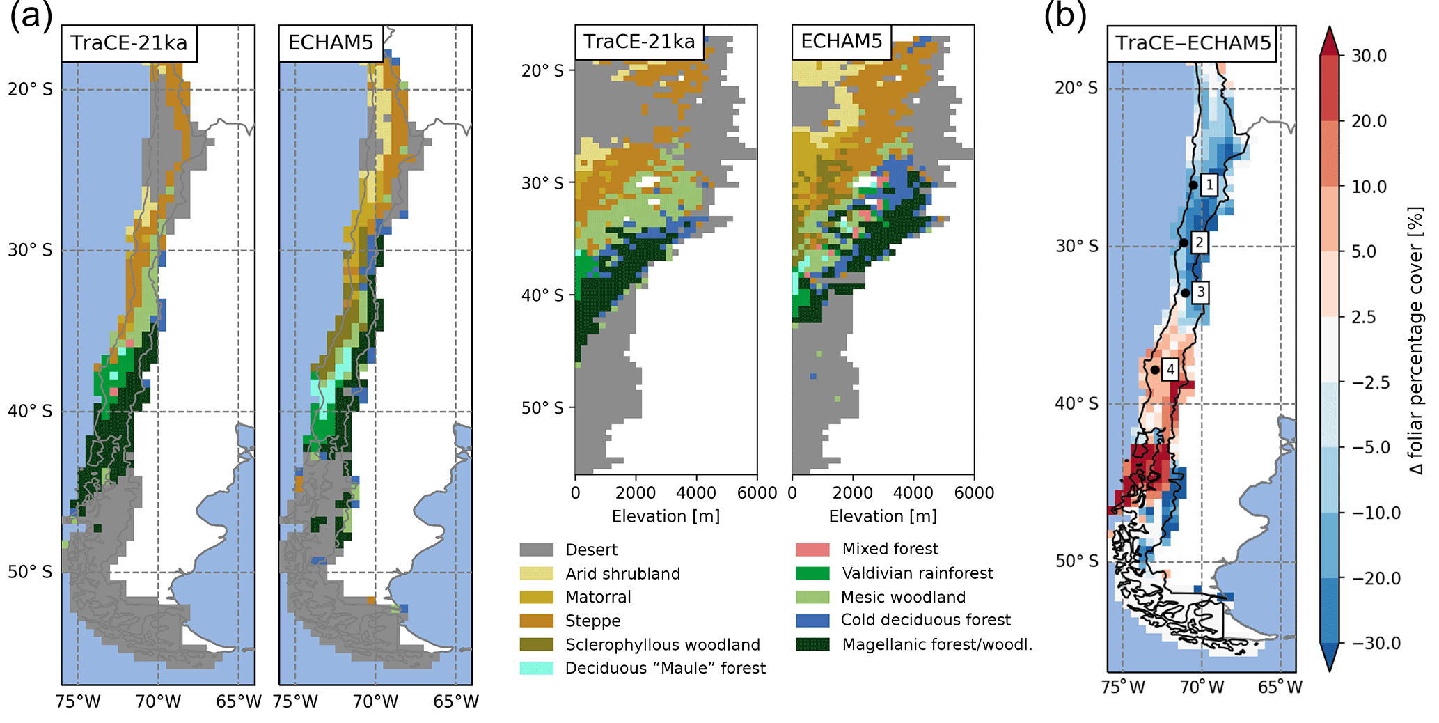
Figure 11(a) The effect of paleoclimate input data used for LPJ-GUESS simulations on the spatial and altitudinal biome distribution and (b) the effect on simulated foliage projected cover (given as the difference between TraCE-21ka simulation and ECHAM5 simulation results, Mutz et al., 2018). For a comparison of the differences between average temperatures and precipitation between the two climate datasets see Figs. 3 and S3. The number 1 represents Pan de Azúcar, 2 represents Sta. Gracia, 3 represents La Campana, and 4 represents Nahuelbuta.
5.3 Sensitivity of simulation to paleoclimate input data
As demonstrated in this study, climatic forcing of the ecosystem model is crucial for the simulated vegetation composition, biome establishment, and associated vegetation cover and surface runoff, which are key controls of catchment denudation rates (Jeffery et al., 2014). The TraCE-21ka dataset was chosen since, to our knowledge, it is the only available dataset providing continuous transient monthly data. However, the low spatial resolution (T31/) is problematic in resolving regional-scale heterogeneity; therefore, we compare our LGM simulations with a regional paleoclimate model simulation (ECHAM5, resolution: T159/ , Mutz et al., 2018). Although the general latitudinal patterns of temperature deviations from PD are similar to TraCE-21ka, precipitation gradients and regional anomalies during the LGM are stronger (see Fig. 3 for LGM anomaly plot of TraCE-21ka data and Fig. S1a, b for ECHAM5). While LGM precipitation anomalies in TraCE-21ka do not exceed 650 mm, precipitation rates in the ECHAM5 data vary by well over 1500 mm for the Andean highlands from 27 to 35∘ S and the coastal areas from 36 to 53∘ S but are markedly lower for the lower Andes and Tierra del Fuego (Fig. S1b). This leads to a different biome distribution pattern for the LGM (Fig. 11). Due to lower temperatures, the cold deserts extend further north and a small zone of temperate rainforest exists at latitudes from 40 to 42∘ S, whereas Magellanic woodlands are simulated with TraCE-21ka. A zone classified as Magellanic woodland stretches from 30 to 42∘ S along the Andean range which gives way to cold deciduous forest at 28 to 32∘ S at altitude. Temperate deciduous “Maule” forest exists north of 40∘ S and transitions into sclerophyllous woodland extending to 30∘ S, whereas TraCE-21ka results lead to steppe at the lowlands and mesic woodlands at higher altitudes. Higher precipitation levels north of 30∘ S also lead to higher vegetation cover, larger areas of matorral and arid shrubland, and a reduction of desert conditions. This results in substantial differences in simulated foliar projected cover (Fig. 11b). While cover of steppe and mesic woodlands simulated with TraCE-21ka is generally 10 %–20 % higher versus the ECHAM5 simulations, the cover from 35∘ S to the Atacama Desert is substantially lower than ECHAM5 (higher precipitation rates for this region). Cover south of 42∘ S is substantially higher for TraCE-21ka as the colder conditions in ECHAM5 simulations generally prohibit vegetation establishment.
The results show that the choice of paleoclimate data clearly has an influence on the simulated vegetation composition, but the impact on vegetation cover depends on the type and location of change. For instance, forest-to-forest transitions due to changes in temperature can have little effect on FPC, while a different annual precipitation rate in Mediterranean to semi-arid conditions can lead to substantial changes in FPC (Sta. Gracia: +200–500 mm precipitation in ECHAM5 LGM data results in > +20 % FPC; Fig. 8a). Given the results from our study we might severely underestimate episodes of elevated erosion in future coupled model exercises – thus, thorough sensitivity studies will be required.
5.4 Impact of atmospheric CO2 on vegetation cover
The effectiveness of photosynthesis, and the related ability of plants to build up biomass, has a large dependence on [CO2] (Farquhar et al., 1980; Hickler et al., 2015). Increases in vegetation biomass (expressed in LAI) were observed in our simulations but coincide with simultaneous rises in temperature and [CO2] (Fig. 9b–d). As observed in the CO2 sensitivity runs for LGM climate conditions, higher [CO2] concentrations lead to an expansion of vegetated areas at higher elevations and an expansion of forest biomes at the expense of herbaceous vegetation. Such changes and the magnitude of the CO2 effect are consistent with earlier LGM simulations (Harrison and Prentice, 2003; Bragg et al., 2013). These changes suggest that [CO2] could play crucial role in understanding landscape evolution over longer timescales – a factor that again is not considered in previous studies of landscape evolution (i.e., Istanbulluoglu and Bras, 2005; Collins et al., 2004).
The strong limiting role of [CO2] during the LGM is generally accepted, but the extent to which substantial CO2 fertilization effects still occur as concentrations increase and rise beyond the current stage is highly debated (Hickler et al., 2015). However, the LPJ-GUESS model with the enabled nitrogen cycle, and nitrogen limiting CO2 effects, has been shown to generally reproduce experimental observations from “Free Air Carbon Dioxide Enrichment” (FACE) experiments (e.g., Zaehle et al., 2014; Medlyn et at al., 2015; De Kauwe et al., 2017). Enabling the nitrogen cycle in LPJ-GUESS is crucial if one aims to understand vegetation response and landscape evolution at [CO2] levels above those of the present day, as have occurred in various episodes of Earths' history (i.e., the Miocene).
In general, we were able to show a temporal compatibility of paleovegetation state, vegetation transitions, and simulated vegetation composition using our model (Sect. 5.2). Our results also indicate that the simulated vegetation is strongly influenced by climatic model drivers (see Sect. 5.3) and [CO2], and by feedback mechanisms occurring within the model (i.e., fire return intervals as controlled by climate and the production of fuel). Given the sensitivity of the vegetation cover to the climate forcing, careful consideration must be made regarding paleoclimate data and its characteristics and uncertainties. The TraCE-21ka data does not show high levels of variability, instead exhibiting only gradual changes over time (temperature, atmospheric CO2 concentration); furthermore, the TraCE-21ka data does not display strong, centennial to millennial scale trends (precipitation). In contrast, available proxy data suggest stronger variability, at least locally, although this is difficult to generalize for larger areas (see Sect. 5.2). Regional paleoclimate simulations with a higher spatial resolution might be required to obtain better landscape-scale model forcing. Another approach may be to modify the climate model derived forcing based on proxy data, such as increasing inter- and intra-annual variability within reasonable ranges (e.g., Giesecke et al., 2010).
In this study, we demonstrated how a DGVM can be applied to estimate vegetation features through time. These features can play an important role in the evolution of landforms, and at a spatial and temporal resolution adequate for coupling with LEMs. The simulation also captures vegetation change drivers that are not explicitly represented in simplified vegetation representations used in LEMs to date, such as plant-physiological effects of changing [CO2], fire dynamics that vary greatly with PFT composition, and interaction with soil water resources via different rooting strategies. The sensitivity of landscape evolution to vegetation and climate changes is evaluated in the companion paper by Schmid et al. (2018). Although our two studies stop short of presenting results from a fully coupled (dynamic vegetation and surface process) model, the results we present highlight (a) how much vegetation likely changed in the Coastal Cordillera of Chile since the LGM (this study), and (b) the general sensitivity of topography and erosion rates to the magnitudes of change identified here (Schmid et al., 2018). In future work we will implement a two-way coupling of LPJ-GUESS to Landlab. LPJ-GUESS will be driven by climate data and will produce a continuous dataset of vegetation cover and surface hydrology that is passed to Landlab. Landlab will use this vegetation cover and simulated denudation rates and will provide updated topography (and after a landform classification, updated areal cover of landforms) and the associated soil depth information to LPJ-GUESS. The novel approach of representing sub-grid diversity in vegetation by landforms allows for efficient computation with existing coarse-scale climate data in addition to coupling to LEMs with higher spatial representations of topography.
From the experiments presented here, our main conclusions are as follows:
-
The regionally adapted version of LPJ-GUESS was able to simulate the latitudinal and altitudinal distribution of potential natural vegetation and the satellite-observed vegetation cover for present-day conditions in most areas of Chile.
-
While simulated MH vegetation did not differ substantially compared to PD PNV, simulated vegetation of the LGM indicates a marked northward shift of biome distribution, a reduction of the tree line, and a downward shift of vegetation zones at altitude. Vegetation cover was generally reduced compared to PD conditions and cold and hot desert covered substantially larger areas of the simulation domain.
-
An analysis of the results from a transient site simulation indicate that temperature and [CO2] caused most of the observed shifts in vegetation composition and (in some cases) transitions between biomes over time. A sensitivity study highlighted the impact of “CO2 fertilization” on vegetation cover under LGM climate conditions.
-
Comparisons with proxy data suggest that coarse-scale climatic forcing underestimates centennial to millennial climate variability. A combination of proxy-derived estimates and climate model results or higher-resolution climate models might be necessary to capture such variability.
-
Our results show that vegetation cover in semi-arid to Mediterranean ecosystems responds strongly to changes in precipitation, while changes in climatic conditions for temperate to boreal forest ecosystems also causes a change in vegetation cover, although to a lesser extent.
-
We consider the implementation of a landform classification a feasible tool to (a) mediate between coarse DVM model resolutions and generally higher-resolution LEMs with little computational expense, and (b) to account for sub-grid variability of micro-climate conditions that are otherwise absent from DVM simulations at larger scales. We envision that it will also allow new applications of LPJ-GUESS to research questions where a better representation of vegetation composition and state, especially the heterogeneity of the simulated sub-pixel vegetation, is important.
In summary, we suggest that coupling state-of-the-art dynamic vegetation modeling with LEMs has great potential for improving our understanding of the evolution of landforms. This is due to the fact that DVMs using the landform approach can approximate the spatial heterogeneity observed in the field which is otherwise not represented by standard DVM implementations. The FPC linked to topography structure will likely result in varying denudation rates in the landscape and will thus have the potential to influence landscape evolution. The regional model adaptation and illustrated model improvements are an important step towards applying a coupled model such as this to the EarthShape study area.
Model setup and results are available upon request from the authors.
It is a well-documented problem that climate models, such as CCSM3, have a tendency to overestimate the precipitation frequency in dry regions (e.g., Dai, 2006). Therefore, we parameterize the number of “wet days” (number of days in a month with rainfall greater than 0.1 mm day−1) based on ERA-Interim daily climatology. It is assumed that the daily precipitation in a month follows a gamma distribution, which is determined by the shape and scale parameters (α and β, respectively) as follows:
where xmean is the monthly mean precipitation, and xstd is its standard deviation (day-to-day variability). A characteristic feature of the gamma distribution is its ability to attain two completely different shapes depending on the value of α. If α<1 (typical for dry regions), the probability density attains maximum value at zero precipitation and decreases exponentially towards higher precipitation values, and if α>1 (typical for wet regions), the probability density function has a shape more reminiscent of a Gaussian distribution.
The number of wet days is estimated from the cumulative gamma distribution:
where Γ is the gamma function. The result of this equation is the probability that an observation will fall in the interval [0x]. Hence for our purposes, the number of wet days (nwet) is determined by
where nday is the number of days in a month, and xt is the threshold value for a wet day (0.1 mm day−1).
In our experiments the TraCE-21k climatology influences monthly nwet by modifying xmean at each grid cell. However, due to the poor representation of precipitation frequencies in the TraCE-21ka data, we use a monthly climatology of xstd calculated from ERA-Interim.
LPJ-GUESS, by default, acknowledges within grid cell variability of vegetation using the concept of patches (Smith et al., 2014). A patch represents a subset of the grid cell that is usually in size. Patches are not spatially registered to any particular location within this cell. By definition, they represent an area of 0.1 ha – the assumed maximum area a mature tree might cover. The replication of these patches ensures that stochastic events (i.e., vegetation establishment and mortality, fire) effect only subsets of a grid cell and allow the model to simulate gap-dynamics and succession. Studies usually are configured with n > =100 patch replications to prevent the stochastic events from dominating simulated average grid cell results. In this study we introduce “landforms” into LPJ-GUESS. The aim is to address two problems. First, the default grid cell size (0.5×0.5) does not allow observed landscape heterogeneity to be addressed (i.e., local site conditions, topographic structure of a catchment). While LPJ-GUESS has been applied at higher resolutions, the lack of high-quality environmental forcing for these resolutions often makes this approach impractical. Second, this new approach allows us to link two models of different model resolutions (LPJ-GUESS and climate drivers , LEM Landlab 100×100 m) to approximate the true DEM characteristics into homogeneous landform units that aim to characterize the dominant topographic units within this grid cell. Thus, the landform concept can be used to mediate the information exchange between these two models. In the implemented landform concept we define a set of patch groups for each landform (i.e., a subset of the grid that shares the same topographic features and similar elevation, slope and aspect). The classification is based on a high-resolution elevation model of the grid cell (SRTM1 data, 30 m), but in a future coupled model the high-resolution DEM will be provided and continuously updated by the landscape evolution model coupled to LPJ-GUESS. The model forcing ( climate and soil texture) is modified for the defined landforms of a given grid cell (see also Fig. B1).
B1 Classification of landforms and modification of environmental drivers
In order to classify landforms, we use the elevation and computed slope and aspect of the grid cells of the high-resolution DEM. Furthermore, aspect and slope are used to compute a topographic position index (TPI) – the difference between elevation and the elevation of surrounding positions (focal radius 300 m; see Weiss, 2001). The TPI and slope values are then used to classify positions into discrete topographic classes (here: ridges – TPI > 1 SD, mid-slopes – TPI > −1 SD and TPI < 1 SD and slope > =6∘, valleys – TPI < SD and flats – TPI > −1 SD and TPI < 1 SD and slope < 6∘). These classes are then stratified by elevation intervals to finally form the landforms (the number of landforms per grid cell depends on complexity of the terrain: mean is 17, 25 % quantile is 11, and 75 % quantile is 23). The average elevation, slope, and aspect are then used to adapt the environmental forcing for this landform.
In this study, we adapt the landform surface temperature via the elevation difference of the grid cell elevation EGC and the average elevation of the high-resolution DEM occupied by a landform (ELF). We also adjust the temperature with the global lapse rate γ of −6.5 ∘C km−1.
Furthermore, we adapt the amount of absorbed radiation based on the landform slope, aspect, and the time of the year. The solar declination (δ) at any given day of the year (doy: day of year) is calculated in LPJ-GUESS as follows (Prentice et al., 1993, all angles in radians):
The solar angle at noon is calculated from the latitude (lat) and δ as follows:
The corrected radiation at the landform (RLF) for north or south facing slopes depending on their aspect (ψ) and slope angle (β) is then calculated from the grid cell radiation in LPJ-GUESS (RGC):
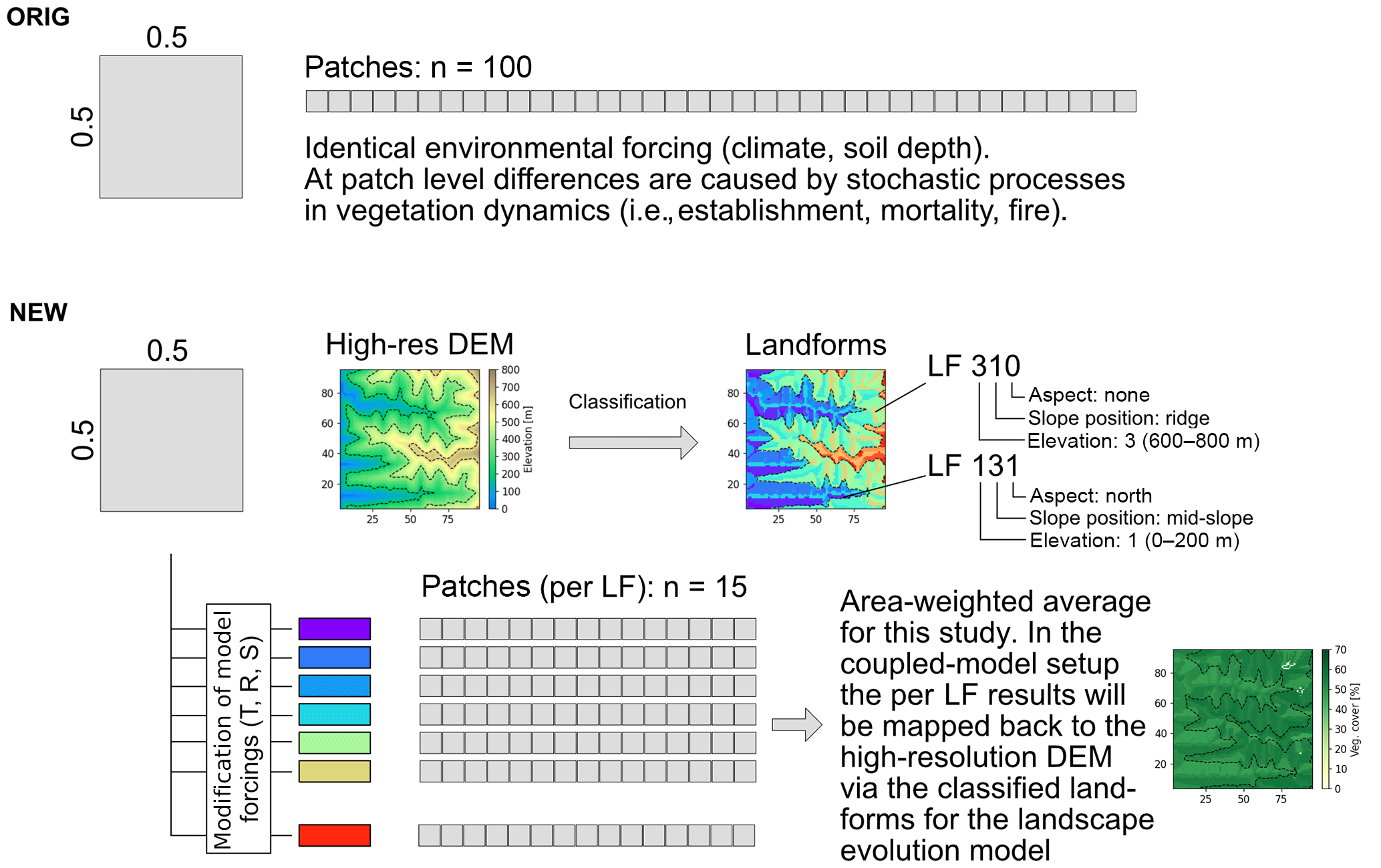
Figure B1Conceptual difference between original LPJ-GUESS patch setup and the new landform addition (T is temperature, R is radiation, S is soil depth, and LF is landform).
Finally, the soil depth of the landform is adjusted based on the TPI of the landform. The default soil depth (DSD) of 1.5 m is scaled by multiplying the height of the lower soil layer (default: 1 m) with fixed values for ridges (0.25), mid-slope positions (0.5), and valleys (1.5) resulting in a total soil depth of 0.75, 1, and 2 m, respectively.
In the future coupled model actual soil depth will be provided by the landscape evolution model.
B2 Model setup with landforms
Instead of running LPJ-GUESS with one environmental condition for all n patches (n > =100) of a grid cell, the model is now executed for each landform and its adjusted environmental conditions n times (n=15). In both model setups the grid cell results are reported as the average results over all n patches (Fig. C1). However, in the landform setup the results are reported as area-weighted averages (the area fraction equals landform fraction within the grid cell). Patches within a landform are averaged in the same way as they are in the default model setup. In a model-coupling setup the model results per landform will be disaggregated back onto the high-resolution DEM of the landscape evolution model to provide a spatially explicit vegetation cover.
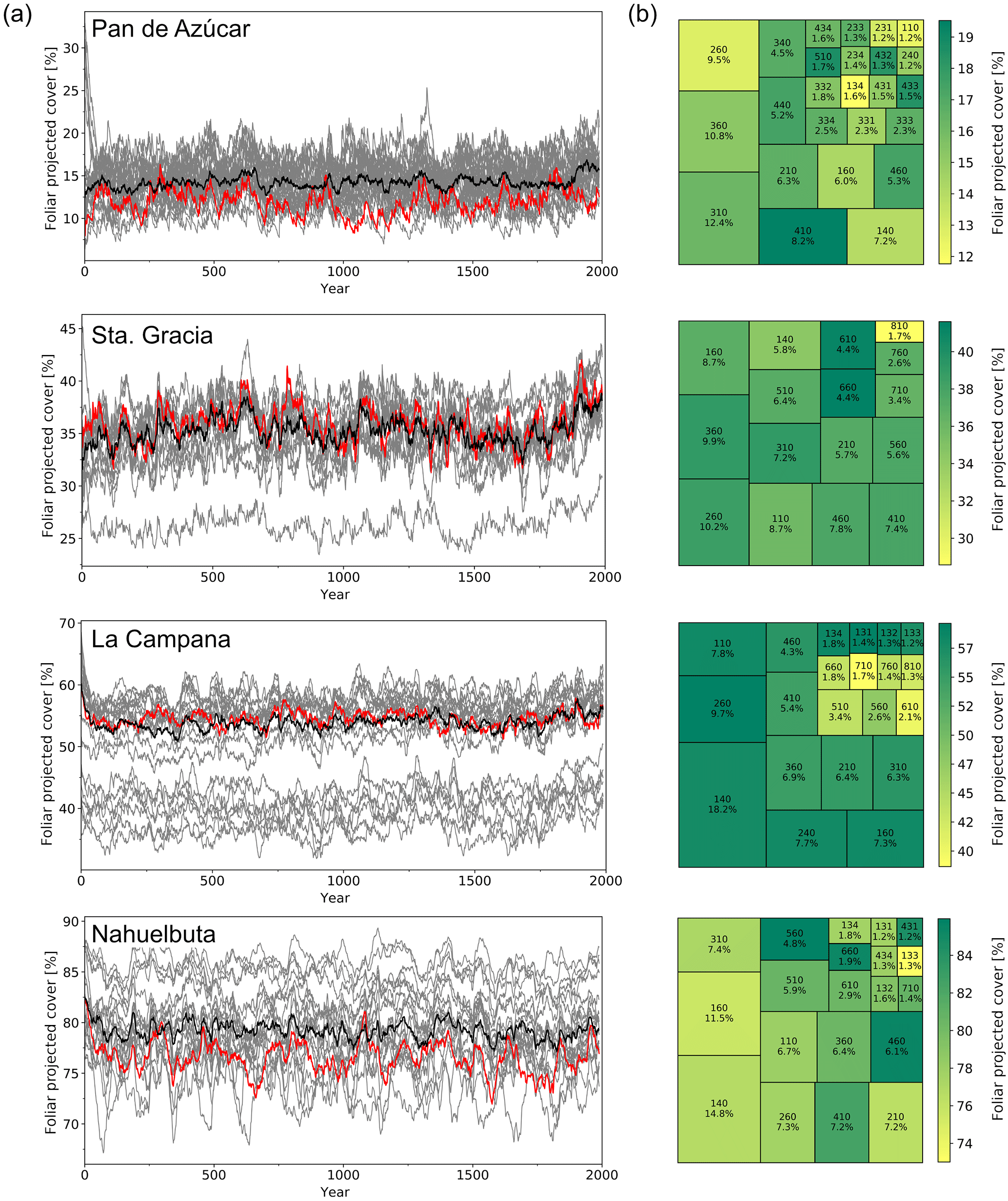
Figure B2(a) Change of foliar projected cover for the individual landforms (gray), the area-weighted mean of all landforms (black), and the default LPJ-GUESS setup with no landforms (red) for the last 2000 years of the transient simulations. (b) Areal extent and foliar projected cover of the individual landforms in the four simulated grid cells (averaged for the last 100 years of the time series; text: landform ID code and percentage of the total grid cell covered by this landform.

Figure C1Flowchart of the decision tree used to classify plant functional types (PFTs) into biomes. LAITOT is the LAI of all PFTs; LAIT is the LAI of tree PFTs; LAIW is the LAI of trees + shrubs; LAIG is the LAI of herbaceous PFTs; LAIX is the LAI of xeric PFTs; LAIB is the LAI of boreal PFTs; fLAIn is the fraction of the LAI PFTn versus its peers (all tree PFTs, boreal PFTs, etc.); TeBE is temperate broad-leaved evergreen trees; TeBS is temperate broad-leaved summergreen trees; BBE is boreal broad-leaved evergreen trees; and BBS is boreal broad-leaved summergreen trees.
Table C1Plant functional type (PFT) characteristics used in this study. Climate classes are associated with differing photosynthesis optimum temperatures and base respiration rates (see Smith et al., 2001; Te is temperate, B is boreal; M is Mediterranean was newly introduced with PS temperatures min: 0, low: 17, high: 27, max: 40; resp. coefficient: 1.0). kallom1 is a constant in allometry equations (Smith et al., 2001; higher values equal wider crowns); Tc,min is the minimum coldest-month temperature for survival; Tc,max is the maximum coldest-month temperature for establishment; GDD5 is the minimum degree-day sum above 5 ∘C for establishment; fAWC is the minimum growing-season (daily temperature > 5 ∘C) fraction of available soil water holding capacity in the first soil layer; rfire is the fraction of individuals that survive fire; kla : sa is the leaf area to sapwood cross-sectional area ratio; z1 is the fraction of roots in first soil layer (the reminder being allocated to second soil layer); aleaf is the leaf longevity; aind is the maximum, non-stressed longevity; CAmax is the maximum woody crown area. r is the base respiration rate (modified after Hickler et al., 2012).
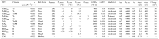
The supplement related to this article is available online at: https://doi.org/10.5194/esurf-6-829-2018-supplement.
Model development, setup, simulations and analysis were conducted by CW. The preparation of the paper was carried out by CW in coordination with TH, MS and TAE, with contributions from all coauthors.
The authors declare that they have no conflict of interest.
This study was funded as part of the German science foundation priority
research program EarthShape: Earth surface shaping by biota (grant no.
EH329-14-1 to Todd A. Ehlers and HI1538/5-1 to Thomas Hickler). We also thank the national
park service of Chile (CONAF) for access to the study areas during field
excursions.
Edited by: Rebecca Hodge
Reviewed by: two anonymous referees
Acosta, V. T., Schildgen, T. F., Clarke, B. A., Scherler, D., Bookhagen, B., Wittmann, H., von Blanckenburg, F., and Strecker, M. R.: Effect of vegetation cover on millennial-scale landscape denudation rates in East Africa, Lithosphere, 7, 408–420, https://doi.org/10.1130/L402.1, 2015.
Allen, J. R. M., Hickler, T., Singarayer, J. S., Sykes, M. T., Valdes, P. J., and Huntley, B.: Last glacial vegetation of northern Eurasia, Quaternary Sci. Rev., 29, 2604–2618, https://doi.org/10.1016/j.quascirev.2010.05.031, 2010.
Armesto, J. J., Arroyo, M. T. K., and Hinojosa, L. F.: The Mediterranean environment of central Chile, in: The Physical Geography of South America, edited by: Veblen, T. T., Young, K. R., and Orme, A. R., Oxford University Press, 184-199, 2007.
Armesto, J. J., Manuschevich, D., Mora, A., Smith-Ramirez, C., Rozzi, R., Abarzua, A. M., and Marquet, P. A.: From the Holocene to the Anthropocene: A historical framework for land cover change in southwestern South America in the past 15 000 years, Land Use Policy, 27, 148–160, https://doi.org/10.1016/j.landusepol.2009.07.006, 2010.
Arroyo, M. T. K., Pliscoff, P., Mihoc, M., and Arroyo-Karlin, M.: The Magellanic moorland, in: The World's Largest Wetlands, edited by: Fraser, L. H. and Keddy, P. A., Cambridge University Press 424–445, 2005.
Batjes, N. H.: ISRIC-WISE Derived soil properties on a 5 by 5 arc-minutes grid (version 1.2), ISRIC Report 2012/01, 2012.
Bonan, G. B.: Forests and climate change: Forcings, feedbacks, and the climate benefits of forests, Science, 320, 1444–1449, https://doi.org/10.1126/science.1155121, 2008.
Bonan, G. B., Levis, S., Kergoat, L., and Oleson, K. W.: Landscapes as patches of plant functional types: An integrating concept for climate and ecosystem models, Global Biogeochem. Cy., 16, 1021–1025, https://doi.org/10.1029/2000GB001360, 2002.
Bragg, F. J., Prentice, I. C., Harrison, S. P., Eglinton, G., Foster, P. N., Rommerskirchen, F., and Rullkötter, J.: Stable isotope and modelling evidence for CO2 as a driver of glacial-interglacial vegetation shifts in southern Africa, Biogeosciences, 10, 2001–2010, https://doi.org/10.5194/bg-10-2001-2013, 2013.
Brook, E.: Windows on the greenhouse, Nature, 453, 291–292, 2008.
Brovkin, V., Raddatz, T., Reick, C. H., Claussen, M., and Gayler, V.: Global biogeophysical interactions between forest and climate, Geophys. Res. Lett., 36, L07405, https://doi.org/10.1029/2009GL037543, 2009.
Bugmann, H.: A review of forest gap models, Climatic Change, 51, 259–305, 2001.
Collins, D. B. G., Bras, R. L., and Tucker, G. E.: Modeling the effects of vegetation-erosion coupling on landscape evolution, J. Geophys. Res.-Earth, 109, F03004, https://doi.org/10.1029/2003JF000028, 2004.
Collins, W. D., Bitz, C. M., Blackmon, M. L., Bonan, G. B., Bretherton, C. S., Carton, J. A., Chang, P., Doney, S. C., Hack, J., James, Henderson, T. B., Kiehl, J. T., Large, W. G., McKenna, D. S., Santer, B. D., and Smith, R. D.: The Community Climate System Model Version 3 (CCSM3), J. Climate, 19, 2122–2143, https://doi.org/10.1175/JCLI3761.1, 2006.
Cramer, W., Bondeau, A., Woodward, F., Prentice, I., Betts, R., Brovkin, V. and, Cox, P., Fisher, V., Foley, J., Friend, A., Kucharik, C., Lomas, M., Ramankutty, N., Sitch, S., Smith, B, White, A., and Young-Molling, C.: Global response of terrestrial ecosystem structure and function to CO2 and climate change: results from six dynamic global vegetation models, Glob. Change Biol., 7, 357–373, https://doi.org/10.1046/j.1365-2486.2001.00383.x, 2001.
Dai, A.: Precipitation characteristics in eighteen coupled climate models, J. Climate, 19, 4605–4630, Precipitation Characteristics in Eighteen Coupled Climate Models, 2006.
Dee, D. P., Uppala, S. M., Simmons, A. J., Berrisford, P., Poli, P., Kobayashi, S., Andrae, U., Balmaseda, M. A., Balsamo, G., Bauer, P., Bechtold, P., Beljaars, A. C. M., Berg, L. van de, Bidlot, J., Bormann, N., Delsol, C., Dragani, R., Fuentes, M., Geer, A. J., Haimberger, L., Healy, S. B., Hersbach, H., Hólm, E. V., Isaksen, L., Kållberg, P., Köhler, M., Matricardi, M., McNally, A. P., Monge-Sanz, B. M., Morcrette, J. J., Park, B. K., Peubey, C., Rosnay, P. de, Tavolato, C., Thépaut, J. N., and Vitart, F.: The ERA-Interim reanalysis: configuration and performance of the data assimilation system, Q. J. Roy. Meteor. Soc., 137, 553–597, https://doi.org/10.1002/qj.828, 2011.
De Kauwe, M. G., Medlyn, B. E., Walker, A. P., Zaehle, S., Asao, S., Guenet, B., Harper, A. B., Hickler, T., Jain, A. K., Luo, Y., Lu, X., Luus, K., Parton, W. J., Shu, S., Wang, Y.-P., Werner, C., Xia, J., Pendall, E., Morgan, J. A., Ryan, E. M., Carrillo, Y., Dijkstra, F. A., Zelikova, T. J., and Norby, R. J.: Challenging terrestrial biosphere models with data from the long-term multifactor Prairie Heating and CO2 Enrichment experiment, Glob. Change Biol., 23, 3623–3645, https://doi.org/10.1111/gcb.13643, 2017.
Diaz, F. P., Latorre, C., Maldonado, A., Quade, J., and Betancourt, J. L.: Rodent middens reveal episodic, long-distance plant colonizations across the hyperarid Atacama Desert over the last 34 000 years, J. Biogeogr., 39, 510–525, https://doi.org/10.1111/j.1365-2699.2011.02617.x, 2012.
Dimiceli, C., Carroll, M., Sohlberg, R., Kim, D. H., Kelly, M., and Townshend, J. R. G.: MOD44B MODIS/Terra Vegetation Continuous Fields Yearly L3 Global 250m SIN Grid V006. 2015, distributed by NASA EOSDIS Land Processes DAAC, doi.org/10.5067/MODIS/MOD44B.006, 2015.
Donoso, C. D. O.: Reseña ecologica de los bosques mediterraneos de Chile, Bosque (Valdivia), 4, 117–146, 1982.
Escobar Avaria, C. A.: Simulating current regional pattern and composition of Chilean native forests using a dynamic ecosystem model, Student thesis series INES, available at: http://lup.lub.lu.se/student-papers/record/3877156 (last access: 15 September 2018), 2013.
Farquhar, G. D., von Caemmerer, S, and Berry, J. A.: A biochemical model of photosynthetic CO2 assimilation in leaves of C3 species, Planta, 149, 78–90, https://doi.org/10.1007/BF00386231, 1980.
Forrest, M., Eronen, J. T., Utescher, T., Knorr, G., Stepanek, C., Lohmann, G., and Hickler, T.: Climate-vegetation modelling and fossil plant data suggest low atmospheric CO2 in the late Miocene, Clim. Past, 11, 1701–1732, https://doi.org/10.5194/cp-11-1701-2015, 2015.
Garreaud, R. and Aceituno, P.: Atmospheric circulation and climatic variability, in: The Physical Geography of South America, edited by: Veblen, T. T., Young, K. R., and Orme, A. R., Oxford University Press, 45–59, 2007.
Garreaud, R., Barichivich, J., Christie, D. A., and Maldonado, A.: Interannual variability of the coastal fog at Fray Jorge relict forests in semiarid Chile, J. Geophys. Res., 113, G04011, https://doi.org/10.1029/2008JG000709, 2008.
Garreaud, R., Falvey, M., and Montecinos, A.: Orographic Precipitation in Coastal Southern Chile: Mean Distribution, Temporal Variability, and Linear Contribution, J. Hydrometeorol., 17, 1185–1202, https://doi.org/10.1175/JHM-D-15-0170.1, 2016.
Gerten, D., Schaphoff, S., Haberlandt, U., Lucht, W., and Sitch, S.: Terrestrial vegetation and water balance – hydrological evaluation of a dynamic global vegetation model, J. Hydrol., 286, 249–270, https://doi.org/10.1016/j.jhydrol.2003.09.029, 2004.
Gerten, D., Lucht, W., Schaphoff, S., Cramer, W., Hickler, T., and Wagner, W.: Hydrologic resilience of the terrestrial biosphere, Geophys. Res. Lett., 32, L21408, https://doi.org/10.1029/2005GL024247, 2005.
Giesecke, T., Miller, P. A., Sykes M. T., Ojala, A. E. K., Seppä, H., and Bradshaw, R. H. W.: The effect of past changes in inter-annual temperature variability on tree distribution limits, J. Biogeogr., 37, 1394–1405, https://doi.org/10.1111/j.1365-2699.2010.02296.x, 2010.
Grosjean, M., Van Leeuwen, J. F. N., Van Der Knaap, W. O., Geyh, M. A., Ammann, B., Tanner, W., Messerli, B., Núñez, L. A., Valero-Garcés, B. L., and Veit, H.: A 22 000 14C year BP sediment and pollen record of climate change from Laguna Miscanti (23∘ S), northern Chile, Global Planet. Change, 28, 35–51, https://doi.org/10.1016/S0921-8181(00)00063-1, 2001.
Gyssels, G., Poesen, J., Bochet, E., and Li, Y.: Impact of plant roots on the resistance of soils to erosion by water: a review, Prog. Phys. Geogr., 29, 189–217, https://doi.org/10.1191/0309133305pp443ra, 2005.
Harrison, S. P. and Prentice, C. I.: Climate and CO2 controls on global vegetation distribution at the last glacial maximum: analysis based on palaeovegetation data, biome modelling and palaeoclimate simulations, Glob. Change Biol., 9, 983–1004, https://doi.org/10.1046/j.1365-2486.2003.00640.x, 2003.
Hempel, S., Frieler, K., Warszawski, L., Schewe, J., and Piontek, F.: A trend-preserving bias correction – the ISI-MIP approach, Earth Syst. Dynam., 4, 219–236, https://doi.org/10.5194/esd-4-219-2013, 2013.
Heusser, C. J.: Ice age vegetation and climate of subtropical Chile, Palaeogeogr. Palaeocl., 80, 107–127, 1990.
Hickler, T., Smith, B., Sykes, M. T., Davis, M. B., Sugita, S., and Walker, K.: Using a generalized vegetation model to simulate vegetation dynamics in northeastern USA, Ecology, 85, 519–530, https://doi.org/10.1890/02-0344, 2004.
Hickler, T., Vohland, K., Feehan, J., Miller, P. A., Smith, B., Costa, L., Giesecke, T., Fronzek, S., Carter, T. R., Cramer, W., Kühn, I., and Sykes, M. T.: Projecting the future distribution of European potential natural vegetation zones with a generalized, tree species-based dynamic vegetation model, Global Ecol. Biogeogr., 21, 50–63, https://doi.org/10.1111/j.1466-8238.2010.00613.x, 2012.
Hickler, T., Rammig, A., and Werner, C.: Modelling CO2 impacts on forest productivity, Curr. Forestry Rep., 1, 1–12, https://doi.org/10.1007/s40725-015-0014-8, 2015.
Hobley, D. E. J., Adams, J. M., Nudurupati, S. S., Hutton, E. W. H., Gasparini, N. M., Istanbulluoglu, E., and Tucker, G. E.: Creative computing with Landlab: an open-source toolkit for building, coupling, and exploring two-dimensional numerical models of Earth-surface dynamics, Earth Surf. Dynam., 5, 21–46, https://doi.org/10.5194/esurf-5-21-2017, 2017.
Hopcroft, P. O., Valdes, P. J., Harper, A. B., and Beerling, D. J.: Multi vegetation model evaluation of the Green Sahara climate regime, Geophys. Res. Lett., 44, 6804–6813, https://doi.org/10.1002/2017GL073740, 2017.
Huntley, B., Allen, J. R. M., Collingham, Y. C., Hickler, T., Lister, A. M., Singarayer, J., Stuart, A. J., Sykes, M. T., and Valdes, P. J.: Millennial climatic fluctuations are key to the structure of Last Glacial ecosystems, PLOS One, 8, e61963, https://doi.org/10.1371/journal.pone.0061963, 2013.
Istanbulluoglu, E. and Bras, R. L.: Vegetation-modulated landscape evolution: Effects of vegetation on landscape processes, drainage density, and topography, J. Geophys. Res.-Earth, 110, F02012, https://doi.org/10.1029/2004JF000249, 2005.
Jeffery, M. L., Yanites, B. J., Poulsen, C. J., and Ehlers, T. A.: Vegetation-precipitation controls on Central Andean topography, J. Geophys. Res.-Earth, 119, 1354–1375, https://doi.org/10.1002/2013JF002919, 2014.
Karger, D. N., Conrad, O., Böhner, J., Kawohl, T., Kreft, H., Soria-Auza, R. W., Zimmermann, N. E., Linder, H. P., and Kessler, M.: Climatologies at high resolution for the earth's land surface areas, Scientific Data, 4, 170122, 2017.
Kobrick, M. and Crippen, R.: SRTMGL1: NASA Shuttle Radar Topography Mission Global 1 arc second V003, https://doi.org/10.5067/MEaSUREs/SRTM/SRTMGL1.003, 2017.
Kosmas, C., Danalatos, N. G., and Gerontidis, S.: The effect of land parameters on vegetation performance and degree of erosion under Mediterranean conditions, Catena, 40, 3–17, 2000.
Langbein, W. B. and Schumm, S. A.: Yield of sediment in relation to mean annual precipitation, EOS T. Am. Geophys. Un., 39, 1076–1084, https://doi.org/10.1029/TR039i006p01076, 1958.
Lehnert, L., Thies, B., Trachte, K., Achilles, S., Osses, P., Baumann, K., Schmidt, J., Samolov, E., Jung, P., Leinweber, P., Büdel, B., and Bendix, J.: A case study on fog/low stratus occurrence at Las Lomitas, Atacama Desert (Chile) as a water source for biological soil crusts, Aerosol Air Qual. Res., 18, 254–269, 2018.
Leung, L. R. and Ghan, J., S.: Parameterizing subgrid orographic precipitation and surface cover in climate models, Mon. Weather Rev., 126, 3271–3291, https://doi.org/10.1175/1520-0493(1998)126<3271:PSOPAS>2.0.CO;2, 1998.
Lara, A., Solari, M. E., Del Rosario Prieto, and Peña, M. P.: Reconstrucción de la cobertura de la vegetación y uso del suelo hacia 1550 y sus cambios a 2007 en la ecorregión de los bosques valdivianos lluviosos de Chile (35∘– 43∘30'S). Bosque (Valdivia), 33, 03–04, https://doi.org/10.4067/S0717-92002012000100002, 2012.
Liakka, J., Colleoni, F., Ahrens, B., and Hickler, T.: The impact of climate-vegetation interactions on the onset of the Antarctic ice sheet, Geophys. Res. Lett., 41, 1269–1276, https://doi.org/10.1002/2013GL058994, 2014.
Liu, Z., Otto-Bliesner, B. L., He, F., Brady, E. C., Tomas, R., Clark, P. U., Carlson, A. E., Lynch-Stieglitz, J., Curry, W., Brook, E., Erickson, D., Jacob, R., Kutzbach, J., and Cheng, J.: Transient simulation of last deglaciation with a new mechanism for Bølling-Allerød warming, Science, 325, 310–314, https://doi.org/10.1126/science.1171041, 2009.
Luebert, F. and Pliscoff, P.: Sinopsis bioclimática y vegetacional de Chile, 2Nd Edition, Editorial Universitaria, Santiago, Chile, 384 pp., 2017.
Lovelock, J. E. and Whitfield, M.: Life span of the biosphere, Nature, 296, 561–563, https://doi.org/10.1038/296561a0, 1982.
Maldonado, A. and Villagrán, C.: Climate variability over the last 9900 cal yr BP from a swamp forest pollen record along the semiarid coast of Chile, Quaternary Res., 66, 246–258, https://doi.org/10.1016/j.yqres.2006.04.003, 2006.
Maldonado, A., Betancourt, J. L., Latorre, C., and Villagran, C.: Pollen analyses from a 50 000-yr rodent midden series in the southern Atacama Desert (25∘ 30' S), J. Quaternary Sci., 20, 493–507, https://doi.org/10.1002/jqs.936, 2005.
Marchant, R., Cleef, A., Harrison, S. P., Hooghiemstra, H., Markgraf, V., van Boxel, J., Ager, T., Almeida, L., Anderson, R., Baied, C., Behling, H., Berrio, J. C., Burbridge, R., Björck, S., Byrne, R., Bush, M., Duivenvoorden, J., Flenley, J., De Oliveira, P., van Geel, B., Graf, K., Gosling, W. D., Harbele, S., van der Hammen, T., Hansen, B., Horn, S., Kuhry, P., Ledru, M.-P., Mayle, F., Leyden, B., Lozano-García, S., Melief, A. M., Moreno, P., Moar, N. T., Prieto, A., van Reenen, G., Salgado-Labouriau, M., Schäbitz, F., Schreve-Brinkman, E. J., and Wille, M.: Pollen-based biome reconstructions for Latin America at 0, 6000 and 18 000 radiocarbon years ago, Clim. Past, 5, 725–767, https://doi.org/10.5194/cp-5-725-2009, 2009.
Medlyn, B. E., Zaehle, S., De Kauwe, M. G., Walker, A. P., Dietze, M. C., Hanson, P. J., Hickler, T., Jain, A. K., Luo, Y., Parton, W., Prentice, I. C., Thornton, P. E., Wang, S., Wang, Y.-P., Weng, E., Iversen, C. M., McCarthy, H. R., Warren, J. M., Oren, R., and Norby, R. J.: Using ecosystem experiments to improve vegetation models, Nat. Clim. Change 5, 528–534, https://doi.org/10.1038/nclimate2621, 2015.
Meinshausen, M., Vogel, E., Nauels, A., Lorbacher, K., Meinshausen, N., Etheridge, D. M., Fraser, P. J., Montzka, S. A., Rayner, P. J., Trudinger, C. M., Krummel, P. B., Beyerle, U., Canadell, J. G., Daniel, J. S., Enting, I. G., Law, R. M., Lunder, C. R., O'Doherty, S., Prinn, R. G., Reimann, S., Rubino, M., Velders, G. J. M., Vollmer, M. K., Wang, R. H. J., and Weiss, R.: Historical greenhouse gas concentrations for climate modelling (CMIP6), Geosci. Model Dev., 10, 2057–2116, https://doi.org/10.5194/gmd-10-2057-2017, 2017.
Monnin, E., Indermuhle, A., Dallenbach, A., Fluckiger, J., Stauffer, B., Stocker, T. F., Raynaud, D., and Barnola, J. M.: Atmospheric CO2 concentrations over the last glacial termination, Science, 291, 112–114, https://doi.org/10.1126/science.291.5501.112, 2001.
Monsi, M. and Saeki, T.: On the factor light in plant communities and its importance for matter production, Ann. Bot., 95, 549–567, https://doi.org/10.1093/aob/mci052, 2005.
Montecinos, A. and Aceituno, P.: Seasonality of the ENSO-related rainfall variability in central Chile and associated circulation anomalies, J. Climate, 16, 281–296, https://doi.org/10.1175/1520-0442(2003)016<0281:SOTERR>2.0.CO;2, 2003.
Morales, P., Hickler, T., Rowell, D. P., Smith, B., and Sykes, M. T.: Changes in European ecosystem productivity and carbon balance driven by regional climate model output, Glob. Change Biol., 13, 108–122, https://doi.org/10.1111/j.1365-2486.2006.01289.x, 2007.
Moreira-Muñoz, A.: Plant Geography of Chile, Springer Netherlands, Dordrecht, 2011.
Moreno, P. I. and Videla, J.: Centennial and millennial-scale hydroclimate changes in northwestern Patagonia since 16,000 yr BP, Quaternary. Sci. Rev., 149, 326–337, https://doi.org/10.1016/j.quascirev.2016.08.008, 2016.
Mutz, S. G., Ehlers, T. A., Werner, M., Lohmann, G., Stepanek, C., and Li, J.: Estimates of late Cenozoic climate change relevant to Earth surface processes in tectonically active orogens, Earth Surf. Dynam., 6, 271–301, https://doi.org/10.5194/esurf-6-271-2018, 2018.
O'ishi, R. and Abe-Ouchi, A.: Polar amplification in the mid-Holocene derived from dynamical vegetation change with a GCM, Geophys. Res. Lett., 38, L14702, https://doi.org/10.1029/2011GL048001, 2011.
Pappas, C., Fatichi, S., Rimkus, S., Burlando, P., and Huber, M. O.: The role of local-scale heterogeneities in terrestrial ecosystem modeling, J. Geophys. Res.-Biogeosci., 120, 341–360, https://doi.org/10.1002/2014JG002735, 2015.
Pollmann, W.: A long-term record of Nothofagus dominance in the southern Andes, Chile, Aust. Ecol., 30, 91–102, https://doi.org/10.1046/j.1442-9993.2004.01427.x 2005.
Prentice, I. C. and Guiot, J.: Reconstructing biomes from palaeoecological data: a general method and its application to European pollen data at 0 and 6 ka, Clim. Dynam., 12, 185–194, https://doi.org/10.1007/BF00211617, 1996.
Prentice, I. C., Sykes, M. T., and Cramer, W.: A simulation model for the transient effects of climate change on forest landscapes, Ecol. Modell., 65, 51–70, https://doi.org/10.1016/0304-3800(93)90126-D, 1993.
Prentice, I. C., Bondeau, A., Cramer, W., Harrison, S. P., Hickler, T., Lucht, W., Sitch, S., Smith, B., and Sykes, M. T.: Dynamic global vegetation modeling: Quantifying terrestrial ecosystem responses to large-scale environmental change Terrestrial Ecosystems in a Changing World, in: Terrestrial Ecosystems in a Changing World, edited by: Canadell, J. G., Pataki, D. E., Pitelka, L. F., Springer, 175–192, 2007.
Prentice, I. C., Harrison, S. P., and Bartlein, P. J.: Global vegetation and terrestrial carbon cycle changes after the last ice age, New Phytol., 189, 988–998, https://doi.org/10.1111/j.1469-8137.2010.03620.x, 2011.
Raddatz, T. J., Reick, C. H., Knorr, W., Kattge, J., Roeckner, E., Schnur, R., Schnitzler, K.-G., Wetzel, P., and Jungclaus, J.: Will the tropical land biosphere dominate the climate–carbon cycle feedback during the twenty-first century?, Clim. Dynam., 29, 565–574, https://doi.org/10.1007/s00382-007-0247-8, 2007.
Reick, C. H., Raddatz, T., Brovkin, V., and Gayler, V.: Representation of natural and anthropogenic land cover change in MPI-ESM, J. Adv. Model. Earth Syst., 5, 459–482, https://doi.org/10.1002/jame.20022, 2013.
Riebe, C. S., Kirchner, J. W., Granger, D. E., and Finkel, R. C.: Minimal climatic control on erosion rates in the Sierra Nevada, California, Geology, 29, 447–450, https://doi.org/10.1130/0091-7613(2001)029<0447:MCCOER>2.0.CO;2, 2001.
Rundel, P. W., Villagra, P. E., Dillon, M. O., Roig-Juñent, S., and Debandi, G.: Arid and semi-arid ecosystems, in: The Physical Geography of South America, edited by: Veblen, T. T., Young, K. R., and Orme, A. R., Oxford University Press, 158–183, 2007.
Schmid, M., Ehlers, T. A., Werner, C., Hickler, T., and Fuentes-Espoz, J.-P.: Effect of changing vegetation and precipitation on denudation – Part 2: Predicted landscape response to transient climate and vegetation cover over millennial to million-year timescales, Earth Surf. Dynam. Discuss., 6, 859–881, https://doi.org/10.5194/esurf-6-859-2018, 2018.
Seiler, C., Hutjes, R. W. A., Kruijt, B., Quispe, J., Añez, S., Arora, V. K., Melton, J. R., Hickler, T., and Kabat, P.: Modeling forest dynamics along climate gradients in Bolivia, J. Geophys. Res.-Biogeosci., 119, 758–775, https://doi.org/10.1002/2013JG002509, 2014.
Seiler, C. R., Hutjes, W. A., Kruijt, B., and Hickler, T.: The sensitivity of wet and dry tropical forests to climate change in Bolivia, J. Geophys. Res.-Biogeosci., 120, 399–413, https://doi.org/10.1002/2014JG002749, 2015.
Sexton, J. O., Song, X.-P., Feng, M., Noojipady, P., Anand, A., Huang, C., Kim, D.-H., Collins, K. M., Channan, S., DiMiceli, C., and Townshend, J. R.: Global, 30-m resolution continuous fields of tree cover: Landsat-based rescaling of MODIS vegetation continuous fields with lidar-based estimates of error, Int. J. Digit. Earth, 6, 427–448, https://doi.org/10.1080/17538947.2013.786146, 2013.
Shellito, C. J. and Sloan, L. C.: Reconstructing a lost Eocene Paradise, Part II: On the utility of dynamic global vegetation models in pre-Quaternary climate studies, Glob. Planet. Change, 50, 18–32, https://doi.org/10.1016/j.gloplacha.2005.08.002, 2006.
Smith, B., Prentice, I. C., and Sykes, M. T.: Representation of vegetation dynamics in the modelling of terrestrial ecosystems comparing two contrasting approaches within European climate space, Global Ecol. Biogeogr., 10, 621–637, https://doi.org/10.1046/j.1466-822X.2001.t01-1-00256.x, 2001.
Smith, B., Wårlind, D., Arneth, A., Hickler, T., Leadley, P., Siltberg, J., and Zaehle, S.: Implications of incorporating N cycling and N limitations on primary production in an individual-based dynamic vegetation model, Biogeosciences, 11, 2027–2054, https://doi.org/10.5194/bg-11-2027-2014, 2014.
Snell, R. S., Huth, A., Nabel, J. E., Bocedi, G., Travis, J. M., Gravel, D., Bugmann, H., Gutiérrez, A. G., Hickler, T., Higgins, S. I., Reineking, B., Scherstjanoi, M., Zurbriggen, N., and Lischke, H.: Using dynamic vegetation models to simulate plant range shifts, Ecography, 37, 1184–1197, https://doi.org/10.1111/ecog.00580, 2014.
Sternberg, M. and Shoshany, M.: Influence of slope aspect on Mediterranean woody formations: Comparison of a semiarid and an arid site in Israel, Ecol. Res., 16, 335–345, https://doi.org/10.1046/j.1440-1703.2001.00393.x, 2001.
Thompson, L. G., Mosley-Thompson, E., Davis, M. E., Lin, P. N., Henderson, K. A., Cole-Dai, J., Bolzan, J. F., and Liu, K.-B.: Late Glacial Stage and Holocene tropical ice core records from Huascarán, Peru, Science, 269, 46–50, https://doi.org/10.1126/science.269.5220.46, 1995.
Thonicke, K., Venevsky, S., Sitch, S., and Cramer, W.: The role of fire disturbance for global vegetation dynamics: coupling fire into a Dynamic Global Vegetation Model, Glob. Ecol. Biogeogr., 10, 661–677, https://doi.org/10.1046/j.1466-822X.2001.00175.x, 2001.
Uribe, J. M., Cabrera, R., de la Fuente, A., and Paneque M: Atlas Bioclimático De Chile, Santiago, Universidad de Chile, 2012.
Valero-Garcés, B. L., Jenny, B., Rondanelli, M., Delgado-Huertas, A., Burns, S. J., Veit, H., and Moreno, A.: Palaeohydrology of Laguna de Tagua Tagua (34∘ 30′ S) and moisture fluctuations in Central Chile for the last 46 000 yr, J. Quaternary Sci., 20, 625–641, https://doi.org/10.1002/jqs.988, 2005.
Vanacker, V., von Blanckenburg, F., Govers, G., Molina, A., Poesen, J., Deckers, J., and Kubik, P: Restoring dense vegetation can slow mountain erosion to near natural benchmark levels, Geology, 35, 303–306, https://doi.org/10.1130/G23109A.1, 2007.
Vaughan, W. W.: Basic atmospheric structure and concepts, Standard Atmosphere, 12–16, 2015.
Veblen, T. T.: Temperate forests of the Southern Andean region, in: The Physical Geography of South America, edited by: Veblen, T. T., Young, K. R., and Orme, A. R., Oxford University Press, 217–231, 2007.
Veblen, T. T., Donoso, C., Kitzberger, T., and Rebertus, A. J.: Ecology of southern Chilean and Argentinean Nothofagus forests, in: The ecology and biogeography of Nothofagus forests, edited by: Veblen, T. T., Hill, R. S., and Read, J., Yale University Press, 293–253, 1996.
Villa-Martínez, R., Villagran, C., and Jenny, B.: The last 7500 cal yr B.P. of westerly rainfall in Central Chile inferred from a high-resolution pollen record from Laguna Aculeo (34∘ S), Quaternary Res., 60, 284–293, https://doi.org/10.1016/j.yqres.2003.07.007, 2003.
Villagrán, C. M.: Expansion of Magellanic Moorland during the late Pleistocene: Palynological evidence from northern Isla de Chiloé, Chile, Quaternary Res., 30, 304–314, https://doi.org/10.1016/0033-5894(88)90006-3, 1988.
Villagrán, C. M.: Quaternary history of the Mediterranean vegetation of Chile, in: Ecology and biogeography of Mediterranean ecosystems in Chile, California, and Australia, edited by: Arroyo, M. T. K., Zedler, P. H., and Fox, M. D., Springer New York, 1995.
Weiss, A.: Topographic position and landforms analysis, Poster presentation, ESRI User Conference, San Diego, CA, Vol. 200, 2001.
Wramneby, A., Smith, B., Zaehle, S., and Sykes, M. T.: Parameter uncertainties in the modelling of vegetation dynamics – Effects on tree community structure and ecosystem functioning in European forest biomes, Ecol. Modell., 216, 277–290, https://doi.org/10.1016/j.ecolmodel.2008.04.013, 2008.
Wramneby, A., Smith, B., and Samuelsson, P.: Hot spots of vegetation-climate feedbacks under future greenhouse forcing in Europe, J. Geophys. Res., 115, D21119, https://doi.org/10.1029/2010JD014307, 2010.
Young, K. R., Berry, P. E., and Veblen, T. T.: Flora and vegetation, in: The Physical Geography of South America, edited by: Veblen, T. T., Young, K. R., and Orme, A. R., Oxford University Press, 91–100, 2007.
Yu, M., Wang, G., and Chen, H.: Quantifying the impacts of land surface schemes and dynamic vegetation on the model dependency of projected changes in surface energy and water budgets, J. Adv. Model. Earth Syst., 8, 370–386, https://doi.org/10.1002/2015MS000492, 2016.
Zaehle, S., Medlyn, B. E., De Kauwe, M. G., Walker, A. P., Dietze, M. C., Hickler, T., Luo, Y., Wang, Y.-P., El-Masri, B., Thornton, P., Jain, A., Wang, S., Wårlind, D., Weng, E., Parton, W., Iversen, C. M., Gallet-Budynek, A., McCarthy, H., Finzi, A., Hanson, P. J., Prentice, I. C., Oren, R., and Norby, R. J.,: Evaluation of 11 terrestrial carbon-nitrogen cycle models against observations from two temperate Free-Air CO2 Enrichment studies, New Phytol., 202, 803–822, https://doi.org/10.1111/nph.12697, 2014.
- Abstract
- Introduction
- Background
- Methods
- Results
- Discussion
- Conclusions
- Data availability
- Appendix A: Calculation of monthly wet days
- Appendix B: Implementation of landforms in LPJ-GUESS
- Appendix C: Plant functional type setup and biomization scheme
- Author contributions
- Competing interests
- Acknowledgements
- References
- Supplement