2.1 Bank erosion cycle

Bank erosion may consist of three phases (Thorne and Tovey, 1981): fluvial entrainment of near-bank riverbed and bank material, mass failure, and disintegration and removal of slump blocks. These three phases are particularly important for cohesive banks since their retreat is typically delayed by the protection offered by slump blocks at their toe (Thorne, 1982; Lawler, 1992; Parker et al., 2011). The waste material settles at the bank toe where it remains for a time depending on its resistance to fluvial erosion and on the available capacity to transport the blocks. In contrast, loose waste material from non-cohesive banks is generally transported away relatively quicker by the river flow, leaving the bank sooner unprotected. Entrainment of near-bank bed material and the intact bank face occurs once the bank toe is exposed again (e.g. see Clark and Wynn, 2007), which continues until the collapse of the upper bank. Mass failure occurs due to geotechnical instability, which can be triggered by different factors, such as fluvial bank toe erosion (e.g. Darby et al., 2007) or a rapid drawdown of the river stage (e.g. Thorne and Tovey, 1981; Rinaldi et al., 2004).

Not only the river flow triggers the bank erosion cycle, but other drivers can contribute to it as well. For instance, subaerial processes may weaken the bank and accelerate later fluvial erosion (Lawler, 1992; Kimiaghalam et al., 2015) or also act as direct agents of erosion (Couper and Maddock, 2001). These effects are included in the entrainment phase for the former example and in the mass failure phase for the latter, which, respectively, promote entrainment or deliver material to the bank toe. Figure 1 illustrates the three phases of erosion in schematic cohesive banks. This representation shows a homogeneous soil which undergoes a continuous cycle of erosion with varying water levels.

Bank erosion can be analysed and measured at two different scales, i.e. the fluvial process and the river cross-section. The measurement at the process scale considers the bank face disintegration over time with evidence of erosion phases (Fig. 1): the mechanisms of erosion develop and are captured at the vertical dimension of the bank. The measurement of bank erosion at the cross-sectional scale, which can be referred to as bankline retreat, consists of tracking banklines over time. In this case, the focus is on the planimetric changes of the bank edge and estimations of eroded volumes and sediment yield. The former approach deals with processes and mechanisms (e.g. Rinaldi and Darby, 2008), whereas the latter with landscape development at larger spatial and temporal scales. Bank erosion studies determine the survey method based on their aims and scales of interest, whereas a given methodology constraints the scope of the findings (Massey, 2001; Couper, 2004). Thus, it is important to identify capabilities and limitations of each survey technique in the context of riverbanks, which are inherently steep features with small-scale irregularities independent of the scale of the river.

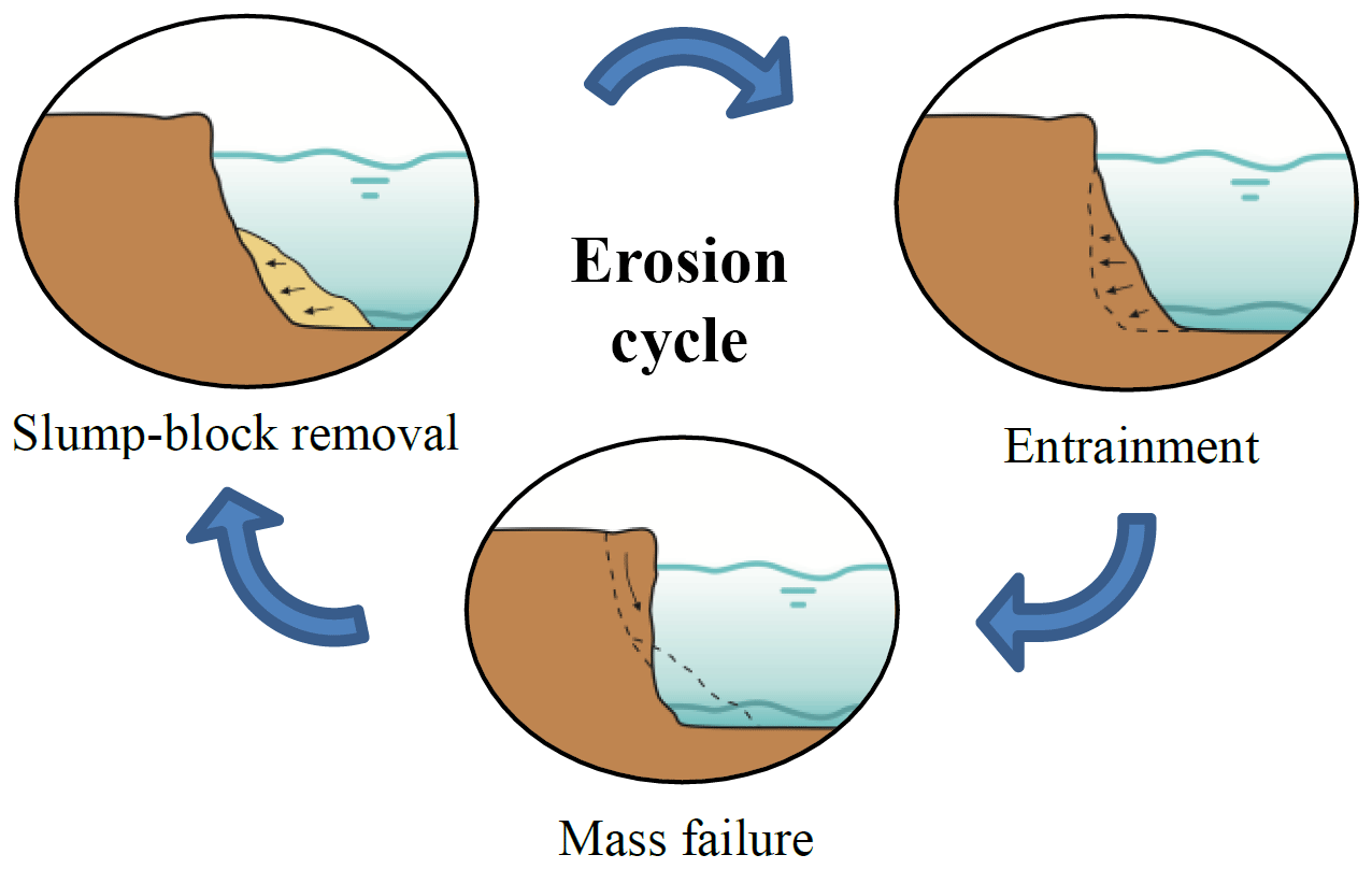
Figure 1Schematic bank erosion phases: slump-block removal (left), entrainment of bare bank (right), and incipient mass failure (centre).

Download

2.2 Techniques to measure bank erosion at different scales

Measuring techniques have four essential characteristics: the extent, resolution, quality, and frequency of measurements. Extent refers to the area or distance along the river covered by each survey; resolution indicates the distance between surveyed points; quality is the precision of position of each surveyed point; and frequency derives from the time interval between consecutive surveys of the same spatial extent or point. The scale of interest may vary among disciplines (e.g. geomorphology, engineering, and ecology), so that diversity of techniques is available with varying spatiotemporal windows of inquiry (Lawler, 1993). Even though the methods currently adopted to measure riverbank erosion range from photo-electric erosion pins to terrestrial laser scanning, they only have high resolution in either time or space (Couper, 2004; Rinaldi and Darby, 2008).

The methods to determine bankline retreat and to estimate eroded volumes are typical of remote sensing, for instance, ALS and aerial photography. The former technique has typical resolutions of 1 and 0.5 m, and covers up to hundreds of square kilometres per day. Bailly et al. (2012) indicate decimetre vertical precision, which depends on several factors including beam footprint size, aircraft inertial measuring system, onboard GPS, vegetation cover, and filtering technique. ALS has been successfully applied to identify river morphological features, such as bar tops (Charlton et al., 2003) and riffle–pool and step–pool sequences (Cavalli et al., 2008; Bailly et al., 2012). In addition, sequential ALS was used to quantify volumes of eroded banks to subsequently estimate pollutant loads, achieving reasonable results for those aims (Thoma et al., 2005). However, banks are particularly steep areas where this technique tends to increase the elevation uncertainty (Bangen et al., 2014). Therefore, banks are regions where lower ALS accuracies are expected compared to horizontal and flat areas.

Bank retreat can be estimated through approaches such as those described by Lawler (1993) that include planimetric resurveys for intermediate timescales (years) and sedimentological and botanical evidence for long timescales (centuries to millennia). Aerial photography interpretation has also been applied to measure bank migration, which is a useful source of information, especially if historical imagery is available over extended periods of time. Nevertheless, it provides only limited information on bank heights, for which this planform survey technique requires other methods to estimate eroded volumes. For example, photogrammetry can serve complementarily to quantify volumetric changes from overlapping photographs (Lane et al., 2010), or ALS to provide recent topographic elevations and reconstruct past morphologies (Rhoades et al., 2009).

Measuring bank erosion at the process scale involves measuring the evolution of the vertical bank profile over time and several other techniques are currently available to that end. Traditional methods include erosion pins and repeated cross-profiling, which provide two-dimensional information with resolutions that, respectively, depend on the number of pins and points across the profile (Lawler, 1993). Erosion pins are simple and effective, but their accuracy may be affected by several factors, such as subaerial processes (Couper et al., 2002). More advanced versions are the photo-electric erosion pins that automatically track the bank face during different erosion phases (Lawler, 2005). Cross-profiling can be done with GPS or total stations with point accuracies of a few centimetres or millimetres, yet with spatial and temporal resolutions that may not be sensitive to very localized or intermittent erosion (e.g. Brasington et al., 2000).

Bank geometries can currently be surveyed at the process scale with their three-dimensional complexity through a number of techniques, whose geomorphic applications are broader than bank erosion studies: terrestrial photogrammetry, terrestrial laser scanning (TLS), boat-based laser scanning, and SfM photogrammetry. Terrestrial photogrammetry has shown detailed bank representations, with approximate resolutions of 2 cm and precision within 3 cm, covering up to 60 m of banks (Barker et al., 1997; Pyle et al., 1997). At the same time, this method can be labour-intensive and requires an accessible bank (Bird et al., 2010), known camera positions and sensor characteristics, and ground-control points, among other considerations (Lane, 2000). TLS has shown detailed erosion patterns from sequential surveys, with millimetre resolutions, which in practice are usually reduced to 2–5 cm, and approximate final accuracies of 2 cm (Resop and Hession, 2010; Leyland et al., 2015). O'Neal and Pizzuto (2011) proved the advantages of 3-D TLS in capturing patterns (e.g. overhanging blocks) and quantifying eroded volumes over 2-D cross-profiling. Even though TLS could cover thousands of metres, in practice, the extents are generally smaller due to accuracy decrease, large incidence angles, occlusion, etc. (Telling et al., 2017), so several scans are necessary to measure long distances. For instance, Brasington et al. (2012) surveyed a 1 km river reach scanning every 200 m along the channel. Alternatively, boat-based laser scanning can continually survey banks with comparable resolutions and accuracies to those of TLS, with great time reduction but involving other field logistics, resources, and post-processing (Alho et al., 2009; Leyland et al., 2017).

3.1 Study site

The study site is a restored reach of the Meuse River, which used to be a single-thread freely meandering river. The river was canalized to a straight reach of 120 m width, the banks were protected, and the water levels regulated to improve navigability. However, several kilometres of banks have been recently restored through the removal of revetments and groynes, following the EU Water Framework Directive 2000/60/EC (http://data.europa.eu/eli/dir/2000/60/oj, last access: 8 January 2018). This reactivated erosion processes to improve the natural value of the river. Important questions have then arisen regarding bank retreat rates and the new equilibrium of the river width. Monitoring bank evolution is necessary to answer these questions and to identify the need, if so, to intervene and at which locations.

The study site is the left bank of a 1200 m long straight reach (Fig. 2) located between the Sambeek and Grave weirs in the southeast Netherlands. This reach presents different bank retreat patterns after 7 years of restoration, with sub-reaches of rather uniform erosion and others with embayments of different lengths. Grassy fields used for grazing cover the riparian zone, followed by crop fields across the floodplain. In the near-bank area, there are poplar trees every 100 m, some of which have been dislodged during the erosion progression, which is possible to appreciate in Fig. 2a considering the ∼200 m embayment between the foreground tree and the next in the background.

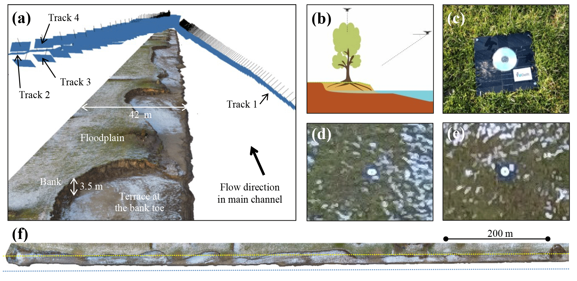
Figure 3(a) Camera positions and orientations in perspective view. The digital surface model shows the low water condition during January 2017, which exposed a terrace at the bank toe. (b) Cross-sectional scheme of UAV paths. (c) Ceramic plaque with CD as ground-control point on the floodplain. (d) GCP in photograph from track 1. (e) Same GCP from track 2. (f) Top view of DSM with UAV track 1 in blue and tracks 2–4 in yellow.

Download

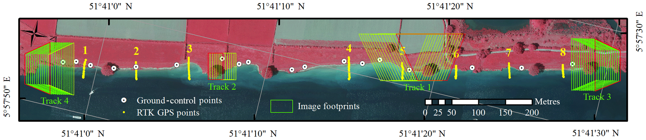
Figure 4Study reach of the Meuse River with GCPs, RTK GPS measurements with cross-section locations and numbers, and some image footprints for all UAV tracks.

Download

The study site was surveyed eight times with the UAV in 2017. An extraordinary low water level in January provided the opportunity to compare the SfM photogrammetry with ALS and RTK GPS not only for the banks and floodplain but also for the sub-aqueous terrace at the bank toe (see schematic cross-sections in Fig. 2). This terrace was composed of bare soil, without vegetation or obstructions, which adds an extra surface for the comparative analysis. This extraordinary exposure was the consequence of a ship accident against the downstream weir of Grave (on 30 December 2016).

3.2 UAV flights for image acquisition

We used the consumer-grade UAV DJI Phantom 4 to take images of the banks. It has a built-in camera with a $\mathrm{1}/{\mathrm{2.3}}^{\prime \prime }$ 12MP sensor and a 94^∘ horizontal angle of view. Prior to the image acquisition, a network of GCPs was distributed on the floodplain to georeference the DSMs (see Fig. 4). The GCPs were spaced approximately every 50 m along the reach, roughly following the tortuous bankline and avoiding proximity to trees, to simplify the field work and facilitate the GCP visibility from the UAV paths (see Figs. 3–4). This approach did not include GCP locations at different elevations, as, for instance, at the bank toe, and relied on the cross-sectional GCP distribution for the stability of the DSM georeferentiation (see Sect. 3.3). The GCPs were 40 by 40 cm black ceramic tiles (Fig. 3c) fixed to the ground with a circular reflector (12 cm CD) at its centre for their fast recognition in the photographs (Fig. 3d–e show how a GCP is seen from tracks 1 and 2). We measured the GCP coordinates using the Leica GS14 RTK GPS unit, which was also deployed for the cross-profiling.

Table 1Number of photographs and overlaps for the tests.

Download Print Version | Download XLSX

An initial flight plan was designed using Universal Ground Control Software (UgCS) to photograph the banks from four different perspectives, to later compare the results of diverse combinations and find a convenient photo set to survey the target topography in subsequent campaigns. The UAV flew four times in straight parallel lines along the banks (Fig. 3a, b, f) to simplify the setup and save flying time, compared to paths that follow changes in bankline or include paths across the domain. The first track took oblique photos from above the river at a height of 25 m and an average (oblique) distance to the bank of 40 m (∼25 m from the least retreated bankline). The second track had a top view from 40 m above the floodplain level along the tree line (Figs. 2–4). The third and fourth tracks followed the same path as the second one in respective upstream and downstream directions, but the camera angle was 50^∘ forward inclined from the horizontal plane (see photo footprints in Fig. 4). These perspectives were thought to capture the tortuous and complex bank surface (Figs. 2, 3a, and 4), including undermined upstream- and downstream-facing scarps, with an average ground resolution of 2.1 cm per pixel. We considered a minimum resolution and accuracy of 1∕25 times the bank height of the river as a requirement to detect erosion processes, which resulted in a maximum acceptable precision of 14 cm for the maximum bank height of 3.5 m at the case study.

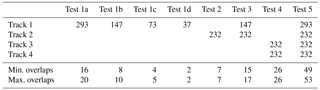
We tested five specific combinations of photographs from the different UAV tracks. Test 1 corresponds to the photo set of the first track only, which has the side view with the optimal coverage of the bank. Test 2 shows for the nadir view alone, which is similar to the viewpoint of classic aerial photography. Test 3 is a combination of the previous two sets. Test 4 combines tracks 3 and 4, i.e. both paths from above the bank with the oblique forward perspectives in upstream and downstream directions, which allows views on all parts of the irregular banks. Finally, test 5 utilizes the four tracks with all photographs (Table 1).

We also used the first oblique track to evaluate the minimum longitudinal photo overlap to efficiently capture the bank relief. The photo overlap along the river is a function of the UAV speed and distance to the bank, for a given maximum photo sampling frequency, which in the case of the deployed UAV is one every 2 s. Then, flying at 2 m s⁻¹ along track 1 resulted in 20 photo overlaps for the most retreated areas and 16 for those zones with least bank retreat, which corresponds to 95 % and 93.7 % image overlap, respectively. Afterwards, in the processing phase, we successively selected a decreasing number of overlaps by twos that resulted in four DSMs. These were test 1a when using all photos from track 1 (which is the same set as the aforementioned test 1), test 1b when using half of them, and so forth for test 1c and test 1d (see Table 1).

3.3 SfM workflow

The principles of SfM photogrammetry are similar to those of digital photogrammetry, but camera positions and lens characteristics are not specified in the former to reconstruct 3-D structures. The camera extrinsic and intrinsic parameters are automatically estimated via tracking and matching pre-defined features in overlapping photos and an iterative bundle adjustment procedure, which results in a sparse point cloud (Hartley and Zisserman, 2003; Snavely et al., 2008; Westoby et al., 2012). Afterwards, the (dense) point matching is done at pixel scale to generate a detailed point cloud of the scene that has the final survey resolution.

GCPs are commonly used to reference the model to a geographical coordinate system, to compute erosion rates and processes through sequential surveys. The georeferencing process involves the Helmert transformation of the point cloud through seven parameters that adjust its scale, position, and rotation in a linear and rigid way (Fonstad et al., 2013). The estimation of these parameters is done through a least-squares regression with the GCPs identified in the UAV images. The propagation of linear errors is thus given by the accuracy with which the GCPs were measured (in this study with the RTK GPS) and then identified in the photographs. Further in the workflow, GCPs can be used to refine the camera parameters estimated during the bundle adjustment, to reduce the non-linear errors that the estimation of the camera parameters may induce. Ideally, well-distributed, precisely measured, and accurately identified GCPs avoid excessive linear and non-linear errors in the point cloud. Yet, a third type of error given by the automated image matching process cannot be prevented with GCPs. These are local and random errors and represent the classic concept of precision.

We used Agisoft PhotoScan software to process the imagery. The camera yaw, pitch, and roll recorded during the UAV flight from different perspectives (Table 1) were input to ensure that the image matching assigned all photos into a single model (Stöcker et al., 2015). For this step, we used three GCPs along the reach, two at the extremes and one in the middle, all close to the bank and easily visible from tracks 1 and 2. These approximate orientations and a priori known ground points helped obtain a consistent sparse point cloud of the bank along the entire reach. The resulting camera positions and orientations of the photo alignment are visible in Fig. 3a, evidencing the UAV tracks. This figure also shows the DSM textured with colours from the photographs, in which the green area on the left side with white patches corresponds to the floodplain partially covered with snow (see also Fig. 3d–f) and the right brownish area is the terrace at the bank toe, with snow remains as well.

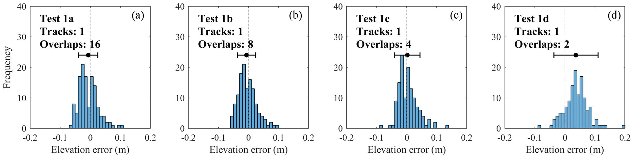
Figure 5Elevation error distributions for SfM tests 1a, 1b, 1c, and 1d, assuming that the RTK points are correct and without error. Indicated overlaps are the minimum.

Download

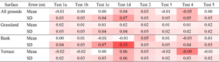
Table 2Mean and standard deviation of elevation differences between SfM DSMs and GPS points. Colour intensity indicates the deviation from zero value with minimum/maximum of ±0.13 m.

Download Print Version

After obtaining the sparse point cloud, we identified the remaining 15 GCPs (Fig. 4) in the photographs, helped by their estimated locations in the model. Then, we refined the camera parameters by minimizing the sum of GCP reprojection and misalignment errors, i.e. using the camera optimization option in PhotoScan. This adjusts the estimated point cloud by reducing non-linear deformations. Once the dense point cloud was computed, we removed the points outside the area of interest, as well as those points at the water surface, tree canopies, and individual bushes at the floodplain. Finally, the point cloud was triangulated and interpolated to generate a TIN, through the arbitrary surface option and the highest number of mesh faces suggested in PhotoScan. This mesh consisted of a non-monotonic surface that was later processed in MATLAB to plot 2-D cross-sections.

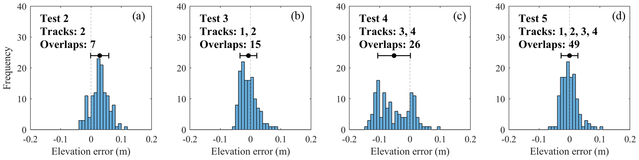
Figure 6Elevation error distribution for tests 2, 3, 4, and 5. Ordinates indicate number of GPS points in each bin.

Download

4.1 DSM precision: identifying necessary photographs

The sequentially decreasing photo overlaps of Track 1 (Table 1) produced four DSMs, tests 1a–1d, whose elevation differences with the 129 RTK GPS points are presented in the histograms of Fig. 5. The elevation errors mostly ranged within 10 cm in all tests, but the mean and standard deviation (SD) presented some differences (Table 2 and dot with bar in Fig. 5). Tests 1a, 1b, and 1c presented mean values smaller than 1 cm and SD within 3–4 cm, while for test 1d these values increased to 4 cm and 7 cm, respectively (Table 2, rows 1–2). The mean errors on the bank area alone for tests 1a, 1b, and 1c were lower than 1 cm (Table 2, row 5), but test 1c had a higher SD of 7 cm compared to 4 and 3 cm of tests 1a and 1b, respectively (Table 2, row 6). Then, tests 1a and 1b had the highest precisions and showed little error differences between them: less than 1 cm for all values in Table 2. Consequently, test 1b with eight photo overlaps was as effective as test 1a with 16 overlaps to achieve the highest DSM accuracy. In addition, test 1b fully covered the tortuous bank area in contrast to test 1c, especially at the perpendicular stretches of embayments (Fig. 3–4), which assured the choice of eight image overlaps over four, despite the general close performance of the latter in terms of accuracy (Table 2, all rows). Therefore, test 1b became the reference for test 1 and was used in combination with test 2 to generate test 3.

Figure 6 shows the error distributions of the remaining four DSMs, i.e. tests 2–5, which also were mostly within 10 cm, except for test 4. This test had evident higher errors than the rest, mostly concentrated at the terrace (Table 2, row 7). Tests 3 and 5 had the lowest mean elevation errors, both lower than 1 cm, with the same SDs at all surfaces that were lower than 3 cm. Test 2 presented a similar SD, but the mean was biased 3 cm. This test in combination with test 1b slightly reduced the SD errors of the latter (Table 2, rows 7 and 6) but without significant overall improvements. All in all, tests 1b, 3, and 5 had the best performance with average errors lower than 1 cm and standard deviations within 3 cm, however, with increasing number of photographs (Table 1). The most efficient one was then test 1b that used the lowest number of photographs to achieve similar precision, especially on banks.

Interestingly, if we consider all tests, the elevation errors on grassland were similar to each other (Table 2, rows 3 and 6), means between 1 and 2 cm, and SD between 2 and 4 cm, whereas the bank and terrace did not present this behaviour. Furthermore, while the bank values (Table 2, rows 4 and 7) did not correlate with those of all grounds (Table 2, rows 1–2), the terrace mean elevation differences (Table 2, row 5) linearly correlated with those of all grounds (Table 2, row 1) with R²=0.97. Therefore, the error biases for all grounds throughout the tests were most likely due to the biases from the points over the terrace.

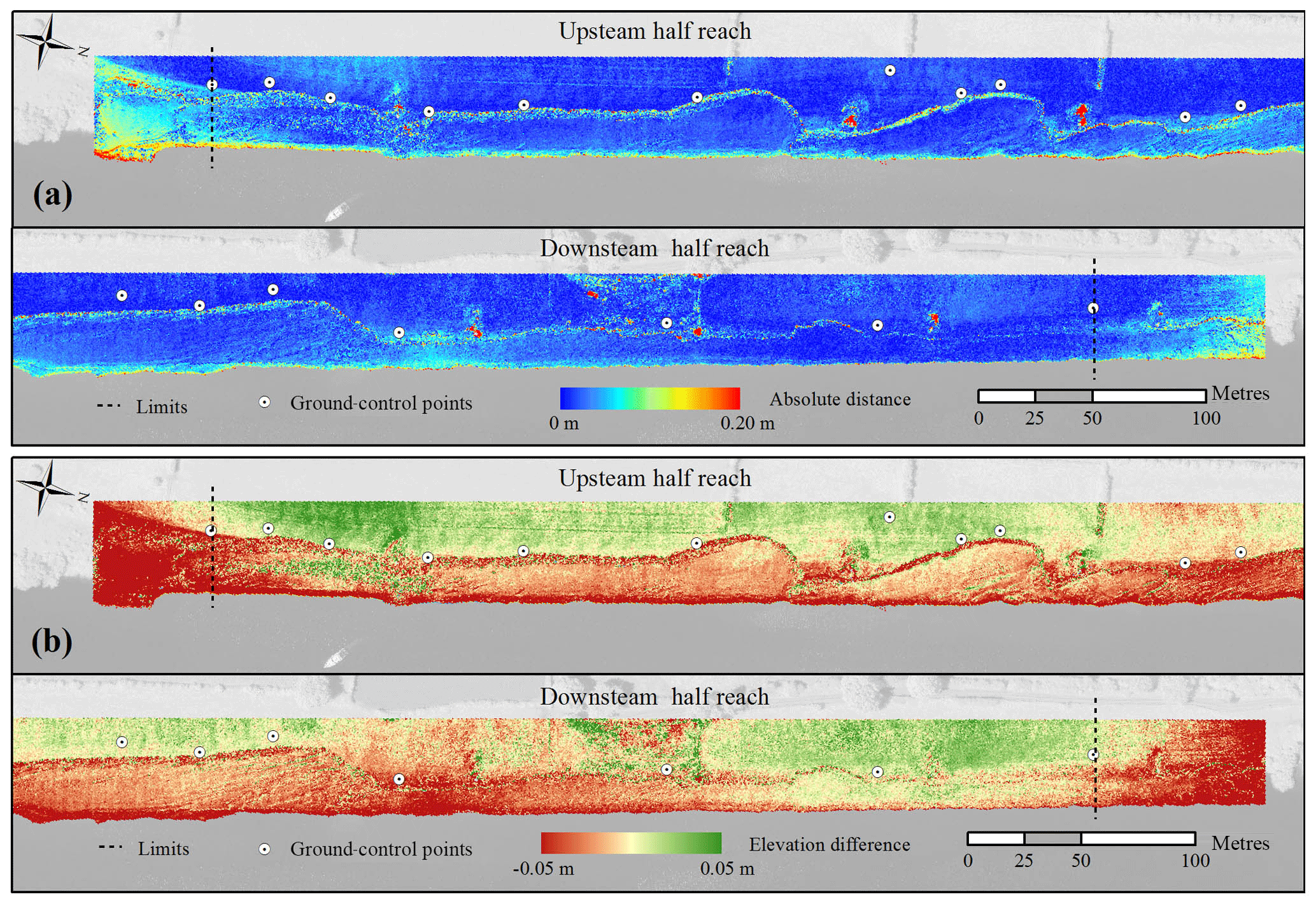
Figure 7(a) Absolute elevation differences between SfM and ALS along the reach. (b) Signed elevation differences between SfM and ALS with a smaller scale range.

Download

To conclude, despite virtually doubling the number of images in comparison with test 1b, the test 3 setup with a nadir track and a side-looking track was chosen for subsequent UAV surveys on the basis of two findings. First, and most important, growing vegetation at the bank toe occluded parts of the target surface from the oblique camera perspective. Second, the GCPs on the floodplain laid almost horizontal, which made them easier to identify from the top view during an initial phase of GCP recognition in the photographs. Moreover, we found at later surveys that growing grass on the floodplain was sometimes blocking GCP plaques from the angle of vision of UAV track 1, for which using the nadir view of track 2 was advantageous to locate the plaque centres, preventing the otherwise disuse of some GCPs.

4.2 DSM precision over the reach: comparison with ALS

Compared to the ALS grid, the test 3 point cloud showed a good agreement over most of the reach. This is observable from Fig. 7a, corresponding to the blue areas that indicate elevation differences lower than 5 cm. However, two notable regions surpassed this difference: the bank and the extremes of the reach. The latter were zones beyond the GCPs, where higher errors in the DSM are expected when using parallel image directions due to inaccurate correction of radial lens distortion (James and Robson, 2014; Smith et al., 2014). Consequently, the results outside the GCP limits were not considered as reliable as those within, where distortion is minimal, and thus were discarded for the subsequent statistical comparisons (beyond the dashed lines in Fig. 7). Within the GCP bounds, the bank area presented relatively high elevation differences, which makes the bankline visible in Fig. 7. Moreover, another sloped area at end of the terrace also presented higher differences than surrounding areas, which is visible as a thin light-blue line at the bottom of the domain in Fig. 7a (see also Fig. 3a–b for other perspectives of this slope toward the channel bed).

Figure 8Comparison of elevation differences between SfM and ALS for distinct surface types.

Download

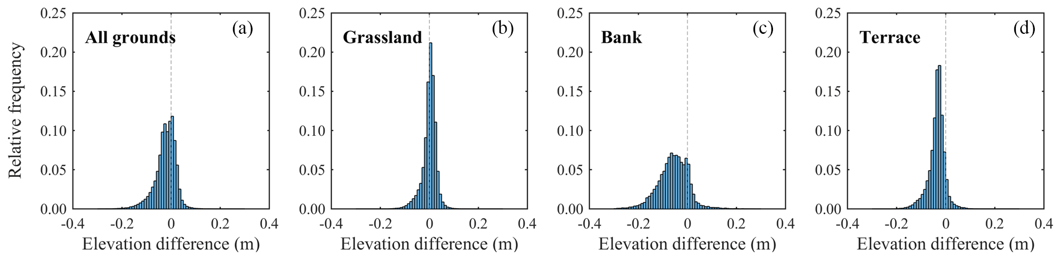
Figure 7b presents signed elevation differences with a smaller scale range to highlight areas with positive and negative deviations between techniques. Green zones indicate higher ground elevations on the SfM DSM than in the ALS grid, red zones indicate the opposite, and yellow shows elevation matches. The upstream half domain presented a general tendency of SfM to overestimate elevations on the floodplain, and in turn underestimate them on the terrace. This trend is also observed in the upper part of the downstream reach. Nevertheless, these zones showed exceptions, such as a green patch at the terrace close to the dashed limit, and a red patch on the floodplain at the end of the upstream half reach. Despite the described general opposed behaviour between floodplain and terrace, the downstream reach evidenced two zones with consistent trends across the domain, covering both the floodplain and terrace. First, lower SfM elevations at the end of the largest embayment (downstream half reach), and second, SfM higher elevations at the end of the reach, before the dashed limit.

Figure 8 presents the relative frequency distributions of the elevation differences divided into three regions: the grassy floodplain, the steep bank, and the bare-ground terrace. Over the grassland, both SfM and ALS had rather similar results (Fig. 8b), with 1 cm mean difference and 2 cm of standard deviation (Table 3). In contrast, the bank had a bias between techniques of 6 cm (Table 3) and a relatively high standard deviation of the same value. Finally, the terrace showed a slightly higher deviation than over the grassland (Fig. 8 and Table 3) but with a bias of −4 cm. The bank area together with the terrace induce an overall small negative bias in the elevation difference distribution (Fig. 8a and Table 3). The former has a small contribution to the total number of measurements and the latter has a greater number but a lower magnitude.

Table 3Mean and standard deviation of elevation differences between SfM, ALS, and RTK GPS. Colour intensity indicates the deviation from zero value with minimum/maximum of ±0.09 m.

Download Print Version

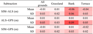
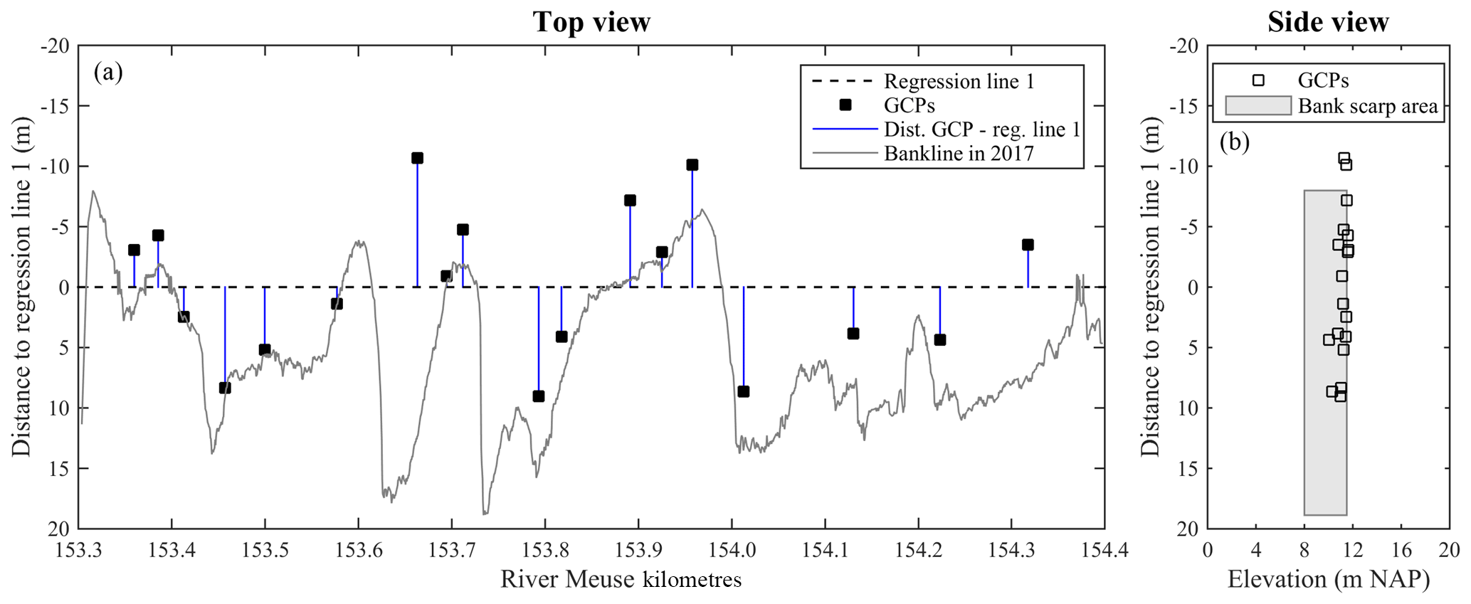
Figure 9GCP horizontal distances to the regression line (a) and respective positions in potential rotation plane from the regression line (b).

Download

Table 3 also indicates the differences of SfM DSM and the ALS with the 129 RTK GPS points. Interestingly, the ALS presented a constant bias of 1 cm across all surfaces, but the standard deviation did change significantly among them: the bank had a standard deviation of 9 cm, which doubled the deviation of the terrace and tripled that of the grassland. While the SfM DSM had comparable absolute biases than those of ALS, the standard deviations were all respectively lower. Particularly at banks, the standard deviation of the SfM DSM was only 3 cm in contrast to the 9 cm of the ALS, which makes the former approach considerably more accurate than the latter. This could explain the relatively large elevation differences between the two methods in the bank area (Fig. 8c) occurring due to a lower precision of the ALS, and not vice versa.

Figure 10(a) Location of GPS measurements in potential rotation plane around regression line 1. (b) SfM DSM elevation errors across regression line 1, distinguished among areas of grassland, bank, and terrace.

Download

4.3 DSM accuracy: rotation around GCP axis

A regression line was computed with the locations of the GCPs to analyse with respect to this axis the rotational tendency of the model. The GCP distributions around the regression line and the bankline are shown in Fig. 9a. The adopted GCPs spanned 19.7 m across the reach and 1.6 m in the vertical direction (Fig. 9, right). The bank scarp along the reach, which is the target survey area, covered 26.9 m in the cross-sectional direction due to the wide-ranging erosion magnitudes of the case study, with maximum bank heights of 3.5 m, indicated with a grey area in Fig. 9b. This side perspective of the domain evidences the potential plane of rotation, whose stability depends on the position of the GCPs.

The rotation potential of the model is evaluated comparing SfM DSM elevations with those of the 129 GPS points (Fig. 4). Figure 10a presents the locations of the GPS points used for accuracy control projected at the potential rotation plane, showing that they covered the domain across the channel (abscissa axis) and different elevations along the scarp area (ordinate axis), resulting in a reasonable sample to assess the model georeferentiation stability. Figure 10b presents the DSM elevation errors distributed across regression line 1. In this plane, a second regression line was computed with all 129 points, represented with a dashed black line in Fig. 10b. This line is tilted from the horizontal suggesting that the model was rotated with a magnitude equal to the respective slope.

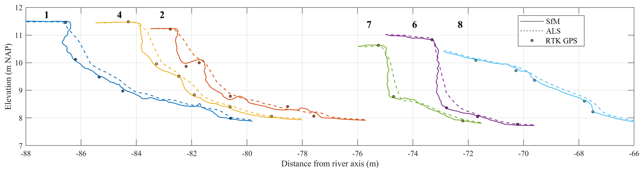
Figure 11Banks measured with SfM (continuous lines), ALS (dashed lines), and GPS (circles) on 17–18 January 2017. Cross-sections are located, from left to right, at river kilometres 153.4, 153.9, 153.5, 154.2, 154.1, and 154.3 (see Fig. 4 for locations).

Download

The GPS points corresponded to difference surface types, shown with different point markers in Fig. 10b. It is clear that on the left side of the regression line 2 down-crossing, errors mostly had a positive bias, whereas on the right they mostly presented a negative bias. At the same time, those errors with positive bias were generally over ground covered with grass, and those with the negative trend were measured on slightly sloped bare ground (see also Table 2, column for Test 3). Then, these tendencies could also be ascribed to the overestimation of the grass cover in the former case and a non-linear transverse deformation beyond the GCP bounds for the latter. Regardless of the causes, the results showed an overall transverse DSM inclination with respect to the GPS points used for accuracy control. Regression line 2, when evaluated at the extremes of the bank scarp area (−7.99 and +18.87 m), yielded an elevation difference between these points of 3.9 cm.

4.4 Bank erosion features and process identification

Six bank profiles were selected among those surveyed with GPS on January 2017 (Fig. 4) to compare the bank representation with the different survey techniques. Figure 11 shows the bank profiles at sections 1, 2, 4, 6, 7, and 8. These sections presented distinct erosion magnitudes and features after 7 years of restoration; for example, section 8 (Figs. 4 and 11) appeared close to the original condition, with a mild slope and nearly no erosion, whereas sections 6 and 7 had vertical scarps. The SfM DSM profiles are represented by continuous lines, the ALS profiles with dashed lines, and GPS points with circles. The SfM representation had better proximity to the GPS points than the ALS in almost all cases. What is more, ALS generally overestimated the elevation corresponding to the GPS points, which confirms the bias observed in the comparison of bank elevations shown in Figs. 7 and 8.

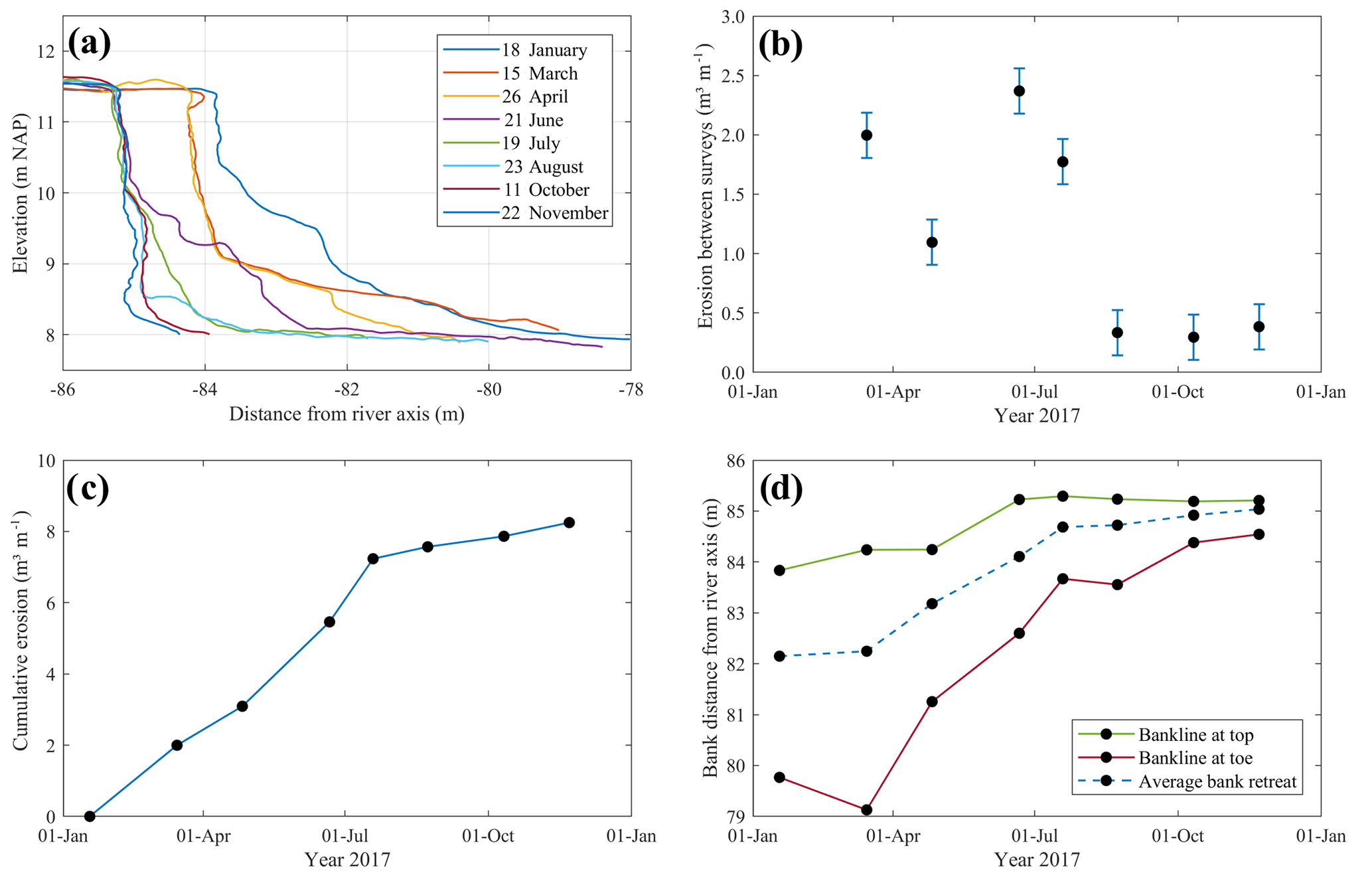
Figure 12Sequential surveys at cross-section 4, Meuse River kilometre 153.9, over 2017. (a) Bank profiles from DSMs; (b) eroded volume per unit width between consecutive surveys; (c) cumulative erosion along surveys; (d) bankline locations at the top and toe of the bank.

Download

SfM profiles showed detailed bank features, such as a collapsed upper bank laying at the toe (section 2), an overhang at the bank top (section 1), small-scale roughness on scarps (sections 6 and 7), and slump-block deposits (section 4). These features appeared as simple shapes in the profiles but they were confirmed with field observations. The ALS depicted simpler profiles, smoothed by coarser resolution, which made it difficult to identify characteristic features of the erosion cycle in them. Yet, ALS profiles had enough point spacing to capture gentle bank slopes with reasonable precision (section 8), but for steeper ones (sections 1, 2, and 4) and especially at scarps (sections 6 and 7), this technique provided lower accuracies.

The temporal development of section 4 (Figs. 4 and 11) is illustrated in Fig. 12a by a sequence of SfM-UAV surveys. The initial stage corresponds to the survey of Fig. 11 on 18 January 2017. The consecutive surveys showed the evolution of the vertical bank profile through which different processes can be inferred. The bank profile, initially characterized by a top short scarp and slump blocks along the bank face, experienced a mass failure and a further removal of blocks between 18 January and 15 March 2017. Between 15 March and 26 April, only toe erosion occurred. By 21 June, another mass failure happened, which left slump blocks along the lower half of the bank. On 19 July, these blocks were removed, leaving a steep bank face. Then, further toe erosion caused a small soil failure at the lower bank whose remains laid at the toe. On 11 October, this wasted material was removed. Then, until the last survey on 22 November, entrainment occurred at the lower half of the bank profile, further steepening the bank. In light of the results, the methodology resolution and accuracy are high enough to identify different phases of the erosion cycle, enabling the analysis of bank erosion processes in conjunction with data on potential drivers.

In addition to process description, eroded volumes can be quantified by computing the net area between sequential bank profiles. For example, Fig. 12b shows eroded volumes per unit width between consecutive surveys plotted at the end of each time interval, with an error bar based on the RMSE of test 3. Evidently, there were different erosion rates during the year and the highest ones happened in the first part of it. Figure 12c presents the respective cumulative eroded volumes per unit width, where the two trends can be distinguished: a gentle slope towards the end and higher rates of sediment yield during the first half of the year. Given that the topographic measurements are limited to a single year, it is not possible to state whether this behaviour is recurrent on a yearly basis. However, this case exemplifies the possibilities to quantify eroded volumes throughout different phases of the erosion cycle.

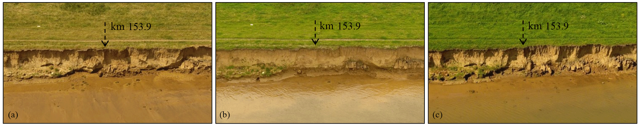
Figure 13Zoomed-in UAV photos from track 1 at section 4, kilometre 153.9, showing diverse bank erosion stages: slump blocks at bank toe on 21 June (a), clean bank face after block removal on 19 July (b), and undermining on 23 August (c).

Download

The bankline retreat as a measure of bank erosion involves the identification over time of the bank top, but this concept could be extended, for instance, to the bank toe. Figure 12d shows the temporal progression of the bankline distance from the river axis for both the bank top and the toe, which we arbitrarily defined for this case at 11.1 and 8.1 m, respectively. The top bankline showed a major jump between April and June and a smaller one between the first two surveys, corresponding to mass failure events. The bank toe presented a more gradual retreat, with events of slumping and temporal accretion that were timely captured along the surveys. This alternative bank retreat representation provides evidence of the development of bank erosion at every survey. The contrast of bankline retreat at the top and toe of the bank illustrates how different processes on their own represent dissimilar erosion evolutions, since they constitute different phases of the erosion cycle, i.e. at the top mass failures and the toe slump-block removal and entrainment. Finally, the average bankline between bank toe and top would best represent the real retreat (dashed line in Fig. 12d), despite not necessarily indicating an actual bank location for a specific elevation. This approach logically considers all erosion phases and follows a similar trend to the cumulative erosion of Fig. 12c.

Finally, the availability of the UAV imagery provides additional information to analyse and interpret bank evolution through direct observation. Figure 13 shows photographs from the three consecutive surveys on 21 June, 19 July, and 23 August at section 4, kilometre 153.9. At this bank area, the sequence shows on the left side of the panels only entrainment at the bank toe, and from the centre (kilometre 153.9) to the right, one or more erosion cycles. Cross-section 4 presented on 21 June (Fig. 13, left panel) slump blocks laying at the bank toe that were removed by 19 July. Then, on 23 August, this cross-section had incipient undermining at the lower bank and block deposition at the toe. The bank area at the right of section 4 experienced a second mass failure after 21 June, completing one erosion cycle, and further downstream it is more difficult to keep track of the cycles due to faster erosion rates. The UAV photos also evidence the progressive growth of grass over the floodplain, especially observable next to the walking path, which was captured along the surveys (Fig. 12a).

5.1 UAV flight and SfM precision

In general, there were no large differences in accuracy between the DSMs derived with different photo perspectives and overlaps. The precision of the tests, except for test 4, was approximately 10 cm complying with the target precision and resolution of 14 cm, and they all represented characteristic features of the erosion cycle, such as slump blocks deposited at the bank toe and mass failures. Other topographic features that were hidden from the nadir UAV perspective, such as undermining, were only captured from oblique camera perspectives. For instance, the area below the top overhangs visible at cross-sections 1 and 2 (Fig. 11) was not captured in test 2 and was represented with a lower resolution in test 4. The UAV viewpoint of track 1 not only had the largest bank area coverage compared to the other camera perspectives proposed in this work but also achieved the highest elevation precision without the need for other tracks. Nevertheless, the nadir view of track 2 contributed to cover an additional bank area behind trees and bushes growing at the bank toe along the first 200 m of the reach (Fig. 2a), for which it was complementarily used with track 1. Since vegetation can occlude the bank face, if denser and more abundant, it could prevent the usage of the survey technique, in a similar way as high water levels do.

The results herein show that, in the absence of bank toe vegetation, a single oblique UAV track with eight photo overlaps and visible GCPs appears effective to survey banks with the highest precision and coverage, for the given sensor size and resolution, camera–object distance, and lighting conditions. This number of photo overlaps agrees with the laboratory experiment of Micheletti et al. (2015), who found that above eight the mean error was only slightly decreased, in contrast to increasing overlaps within the range below eight. Nonetheless, they showed that overlaps higher than eight reduced the number of outliers, a trend which in our case is evident for less overlaps: test 1c (four overlaps) mainly differed from test 1b (eight overlaps) in a higher RMSE but not in the mean. This difference may arise from the distinct texture and complexity of each surface, which presumably requires different number of images for a similar performance (James and Robson, 2012; Westoby et al., 2012; Micheletti et al., 2015).

A RMSE of 2.8 cm to measure a riverbank with the photo combination of test 3 results in a relative precision with respect to the average camera–surface distance of 0.0007 or ∼1 : 1400. This relative precision ratio is somewhat higher than ∼1 : 1000 achieved by James and Robson (2012) for steep irregular features at kilometre scale in a volcanic crater and decametre scale in a coastal cliff, whereas our precision is somewhat lower than ∼1 : 2000, which those authors proved at metre scale. More precise results could be possible using a bigger and higher-resolution sensor, flying closer to the bank, or even trying other oblique bank perspectives. However, this endeavour would only be reasonable if such data are needed for research purposes and if GCP positioning had also according higher precisions, since registration errors translate into the DSM accuracy during camera parameter optimization (Harwin and Lucieer, 2012; Javernick et al., 2014; Smith et al., 2014).

A precision of 10 cm has implications for the representation of small-scale features at bank scarps. Despite the presence of features in the order of decimetres, we could not assess their accuracy given the discrete GPS points and the 0.5 m ALS grid used to assess the DSM precision. For instance, Fig. 12a shows an upper bank scarp along the last four surveys that, if assumed unchanged, would indicate a maximum distance of 20 cm between surveys, which still would remain within the ±10 cm error estimated by the GPS comparison. Although these differences could have been caused by weathering processes or growing grass on the bank face, potential sources of error at such scale could be given, for instance, by registration errors or occlusions caused by the surface roughness (Lague et al., 2013). Then, further research is needed to evaluate the precision at the roughness scale to, for example, analyse form drag at the bank face (Leyland et al., 2015).

The analysis made for test 3 on model rotation evidenced a linear trend with increased surface elevations on the floodplain side of the domain and decreased elevations on the main channel side (Fig. 10b). This tendency was probably caused by a rotation of the DSM around co-linear GCPs that may lead to rotated solutions of the Helmert transformation (Carbonneau and Dietrich, 2017). Yet, the areal SfM-ALS comparison within ±5 cm range (Fig. 7b) did not evidence a clear axis along the whole domain that could suggest a rigid rotation of the DSM, since the ALS did have a constant mean accuracy across all surface types (Table 3). The linear rotation tendency, then, might have been obscured by the error range that was larger across the domain (Figs. 6b and 10b) than the mean rotation magnitude, whose elevation difference between the extremes of the cross-sectional domain was 6 cm, and 4 cm within the bank area. Thus, other sources of error were also present that resulted in the obtained error range.

The comparative analysis of the DSM elevation errors from different photo combinations showed that the ground surfaces surveyed in the case study had different precisions. The grassland presented similar errors with a positive bias throughout all tests. The positive elevation differences are typical of vegetated surfaces (Westoby et al., 2012; Micheletti et al., 2015), whereas the similar performance of different photo combinations might be due to the presence of sufficient and well-distributed GCPs in this area (the floodplain). The terrace at the toe of the bank, in contrast, presented different error skewness throughout the tests, which affected the error distribution for all grounds. Interestingly, the error deviation of test 1 increased as the overlaps decreased, which in turn implies that more overlaps created more robust models. The linear errors cannot explain this behaviour because the same GCP locations were used for all tests, and only the camera parameters were optimized for each.

The error skewness at the terrace throughout the tests could be related to the fact that this area was the most distant from the GCPs and it was not surrounded by them, so that errors in lens distortion corrections could have especially increased here (James and Robson, 2014; Javernick et al., 2014; Smith et al., 2014). This effect was clear at the reach extremes (Fig. 7), where the elevation differences increased with respect to the ALS survey further from the GCPs, for which it is called “dome” effect. While James and Robson (2014) showed that using different (convergent) camera angles is effective to mitigate the “dome” effect, our results showed that the DSM precision with eight photo overlaps along a single UAV track did not substantially improve by adding the extra perspective of track 2. This may imply that the chosen number of overlaps and used GCPs were sufficient to avoid distortions in the bank area that exceed the required accuracy, together with the fact the track had oblique and not nadiral perspective.

It is most likely that all the mentioned types of error were present in the SfM DSM, i.e. linear errors given by rotation (linear trend of errors across potential rotation plane; Fig. 10b), non-linear errors given by the estimation of camera parameters (patches of higher or lower SfM elevations across the domain compared to ALS; Fig. 7b), overestimation of ground elevation with grass cover (Table 2, Figs. 7b, 12a), and random errors given by the bundle adjustment that could not be assessed herein. Although the adopted workflow was effective to measure bank erosion processes with the target accuracy, linear and non-linear errors could have been reduced, for instance, using a larger cross-sectional GCP distribution or better visible and bigger GCP targets. Other possibilities are also open, such as combining two oblique perspectives with a second angle better capturing the floodplain, GCPs, and bank area.

5.2 Comparison of two reach-scale techniques: SfM and ALS

The elevation bias at the bank between the SfM-based DSM and the ALS grid (Fig. 8) was caused by the topographic overestimation of ALS (Table 3 and Fig. 9). This ubiquitous error is ascribed to a known limitation of ALS systems related to the laser beam divergence angle, which locates the closest feature within the laser footprint at the centre of the footprint. This increases the ground elevation at high-slope areas (Bailly et al., 2012), which is the case for riverbanks. Still, the ALS resolution and precision were enough to identify bank slopes, in accordance with other studies (e.g. Tarolli et al., 2012; Ortuño et al., 2017). Furthermore, despite the ALS capability to estimate volume changes of eroded banks (Kessler et al., 2013), the method omits information related to the phases of the erosion cycle by not surveying erosion features smaller than its resolution (in this case, 0.5 m), apparent in contrast with SfM profiles (Fig. 11). Moreover, if finer ALS resolutions are available, for instance, using higher frequency lasers or working with the raw data, more ground details can be captured, but still vertical or undermined profiles would be missed.

The elevation differences between the methods observed for grassland (Fig. 8b) were probably caused by dissimilar ground resolutions, because a larger elevation scatter is expected in the SfM-based DSM when capturing grass with 2 cm resolution, compared to the interpolated ALS samples into a 50 cm grid, even when derived from 0.16 m beam footprints. Nonetheless, the mean difference was zero (Table 3), so that both methods overestimate in the same way the real ground elevation due to grass cover. The effect of this is visible, for instance, in the increasing surface elevations on the floodplain over a year (Fig. 12a), which happens after the mowing period in October. The terrace at the bank toe presented a similar scatter as grassland but had a small negative bias that could be explained by a DSM rotation or a slight transverse “dome” effect of the SfM DSM.

The distance covered by the SfM-UAV method depends on the flight autonomy. The deployed UAV had autonomy of approximately 25 min, which limited the maximum bank survey extent to approximately 2 km for the tested UAV height and speed, and camera resolution and shutter frequency. This practical limit will change with the progressive development of UAVs, but the distance covered by a single flight is currently significantly smaller than the one covered by ALS. Although a larger camera–object distance and speed than those used in this work would increase the surveyed area, decreasing the ground resolution and the UAV stability may result in the loss of sufficient detail to capture erosion features, and what is more, decrease the DSM precision that depends on the image scale (James and Robson, 2012; Micheletti et al., 2015). Therefore, further investigations would be required to explore the practical limits of UAV bank monitoring in views of extending the survey coverage.

5.3 UAV-SfM challenges to measure bank erosion processes

The use of UAV-SfM to measure bank erosion processes presents specific challenges, since bank areas usually have vertical surfaces and lengths can be much larger than the other two dimensions. Furthermore, the reach under analysis was particularly straight, introducing additional complexity to apply the technique.

5.4 Surveying bank erosion with UAV-SfM and other techniques

Sequential surveys allowed to capture different phases of the erosion cycle (Fig. 12a), which demonstrates that quantitative detection of processes is feasible. Previous studies on bank erosion proved the capabilities of SfM for post-event analysis (Prosdocimi et al., 2015), e.g. representing block deposition, or for 2.5-D bank retreat quantification (Hamshaw et al., 2017), whereas herein all erosion phases were sequentially captured, demonstrating the 3-D potentialities over the complete process of erosion. Of course, the ability to monitor banks at the process scale depends on the time interval with which the method can re-survey the exposed part of banks and will only cover pre- and post-flood conditions. The survey frequency and the duration of a full cycle of erosion determine the temporal resolution with which the development of processes is captured. Then, the bank retreat rate of each case determines the necessary frequency of surveys to capture erosion processes within a single cycle. Bank erosion rates naturally depend on each site, after different river sizes, hydraulic conditions, bank materials, etc. In the presented study site, erosion rates varied enormously (Fig. 3), but still the performed eight surveys within a year successfully captured bank processes within a single erosion cycle in areas of fast retreat such as section 4.

The study site with a regulated water level and recently restored actively eroding banks was a perfect example for the application of this technique, because banks were exposed and erosion rates were compatible with the proposed average sampling frequency of 6 weeks. For other types of rivers, where erosion mainly occurs during floods when banks are not exposed, this method would allow measuring pre- and post-event conditions only. Given the high resolution achieved, the method is applicable to all river sizes. However, with the accuracy of the adopted workflow, the application is only advised in cases where bank retreat is larger than approximately 30 cm between consecutive surveys.

Erosion processes happening at small spatial scales, such as weathering, would be hardly or not measurable with the precision achieved in this investigation. For this, other methods are already available, for instance, TLS and boat-based laser scanning, that provide higher precisions (millimetres before registration errors, e.g. O'Neal and Pizzuto, 2011) and comparable resolutions (centimetres; e.g. Heritage and Hetherington, 2007). In addition, close-range terrestrial photogrammetry can also offer the necessary precision for such endeavours, e.g. from a tripod (Leyland et al., 2015) or a pole on the near-bank area (Bird et al., 2010), at the expense of covering shorter bank lengths. Another alternative is erosion pins, which may also provide higher accuracies, yet with point resolution.

UAV-SfM appears a suitable survey method for both process identification and volume quantification in bank erosion studies, given the decimetre precision range with 3 cm RMSE and the 3-D high resolution achieved with a low-cost UAV. As Resop and Hession (2010) suggested, high-resolution three-dimensional capabilities offer great possibilities when spatial variability of retreat is critical compared to traditional cross-profiling methods. In addition, the reduced deployment time of UAVs in the field is advantageous in relation to cross-profiling, while it also improves identification of complex bank features (Fig. 11) and volume computations as other 3-D high-resolution techniques (O'Neal and Pizzuto, 2011). Nonetheless, UAV-SfM requires longer post-processing times at the office, which should not be underestimated (Westoby et al., 2012; Passalacqua et al., 2015).

This technique remains less expensive than TLS or mobile laser scanning (MLS), which is more convenient for cases where roughness is beyond the scale of interest, and target bank lengths are smaller than 3000 m. This would approximately be the longest distance for a single UAV flight in our case study. For longer reaches, MLS would then compete with UAV-SfM from a practical perspective, since more than one survey/flight would be needed. However, all TLS, MLS and UAV-SfM have limitations to survey the bank surface in presence of dense bank vegetation (Hamshaw et al., 2017). In these cases, ALS provides an alternative, albeit with significant lower resolution and higher costs (Slatton et al., 2007).

For large river extents, i.e. several kilometres, Grove et al. (2013) showed that process inference is possible combining ALS with high-resolution aerial photography, two techniques that are typically applied for eroded volume estimations and bank migration (Khan and Islam, 2003; Lane et al., 2010; De Rose and Basher, 2011; Spiekermann et al., 2017). In that work, the scale of the river (banks higher than 6 m) allowed a spatial resolution of 1 m to capture features that together with photo inspection provided information on mass failure type and fluvial entrainment. To date, UAV-SfM covers smaller extents (Passalacqua et al., 2015), but provides much higher resolutions, allowing for process identification (such as undermining) and more precise volume computations (see Fig. 11 for profile differences between ALS and SfM). For a similar (or higher) accuracy and resolution than those of UAV-SfM and large distances, boat-based laser scanning becomes an attractive, but more expensive, solution.