the Creative Commons Attribution 4.0 License.
the Creative Commons Attribution 4.0 License.
 | 14 Mar 2019
How steady are steady-state mountain belts? A reexamination of the Olympic Mountains (Washington state, USA)
Lorenz Michel
Christoph Glotzbach
Sarah Falkowski
Byron A. Adams
Todd A. Ehlers
The Olympic Mountains of Washington state (USA) represent the aerially exposed accretionary wedge of the Cascadia Subduction Zone and are thought to be in flux steady state, whereby the mass outflux (denudation) and influx (tectonic accretion) into the mountain range are balanced. We use a multi-method approach to investigate how temporal variations in the influx and outflux could affect previous interpretations of flux steady state. This includes the analysis of published and new thermochronometric ages for (U–Th) ∕ He dating of apatite and zircon (AHe and ZHe, respectively), fission-track dating of apatite and zircon (AFT and ZFT, respectively), 1-D thermo-kinematic modeling of thermochronometric data, and independent estimates of outflux and influx.
In total, we present 61 new AHe, ZHe, AFT, and ZFT thermochronometric ages from 21 new samples. AHe ages are generally young (< 4 Ma), and, in some samples, AFT ages (5–8 Ma) overlap ZHe ages (7–9 Ma) within uncertainties. Thermo-kinematic modeling shows that exhumation rates are temporally variable, with rates decreasing from > 2 to < 0.3 km Myr−1 around 5–7 Ma. With the onset of Plio–Pleistocene glaciation, exhumation rates increased to values > 1 km Myr−1. This demonstrates that the material outflux varies through time, requiring a commensurate variation in influx to maintain flux steady state. Evaluation of the offshore and onshore sediment record shows that the material influx is also variable through time and that the amount of accreted sediment in the wedge is spatially variable. This qualitatively suggests that significant perturbations of steady state occur on shorter timescales (105–106 years), like those created by Plio–Pleistocene glaciation. Our quantitative assessment of influx and outflux indicates that the Olympic Mountains could be in flux steady state on long timescales (107 years).
- Article
(19933 KB) - Full-text XML
-
Supplement
(7562 KB) - BibTeX
- EndNote


The assumption of a balance between opposing processes has allowed geoscientists to use proxy measurements (like denudation rates) to constrain difficult-to-measure variables like rock uplift. This has given rise to the concept of steady-state landscapes or mountain ranges. Likewise, a steady state (i.e., a mass balance) is commonly one of the boundary conditions in modeling studies investigating the evolution and dynamics of orogens in response to changes of other boundary conditions like climate or tectonic fluctuations (e.g., Batt et al., 2001; Stolar et al., 2007; Whipple and Meade, 2006; Willett, 1999). Two main types of steady state are often used to interpret mountain-building processes (e.g., Willett and Brandon, 2002): (1) topographic steady state, in which the topography is invariant because rock uplift and horizontal motion of material are balanced by denudation, and (2) flux steady state, in which the material influx (by accretion of sediment and rock) is balanced by the material outflux (by denudation) from a mountain range. The assumption of steadiness is both spatial- and timescale-dependent so that for a given timescale, steadiness might only be achieved on a large, orogen-wide spatial scale due to the spatial averaging of single processes acting on a small scale (e.g., catchment-wide sediment discharge vs. orogen-wide sediment discharge). Furthermore, a possible perturbation of steady state is sensitive to the timescale it takes for orogens to respond to variations in crustal deformation or a change in climate. If the timescales required for a change in the influx and outflux are significantly different from each other, a deviation from steady state is likely.
Likewise, studies from different orogens worldwide suggest strong variations in denudation and exhumation on million-year timescales. These variations can be linked to changes in tectonic conditions (e.g., Adams et al., 2015; Lease et al., 2016), the internal dynamics of drainage basins (e.g., Willett et al., 2014; Yanites et al., 2013), changes in the magnitude of precipitation (e.g., Lease and Ehlers, 2013; Whipple, 2009), or the onset of glaciation (e.g., Berger et al., 2008; Bernard et al., 2016; Ehlers et al., 2006; Glotzbach et al., 2013; Gulick et al., 2015; Herman et al., 2013; Herman and Brandon, 2015; Lease et al., 2016; Thomson et al., 2010, 2013; Valla et al., 2011; Yanites and Ehlers, 2012).
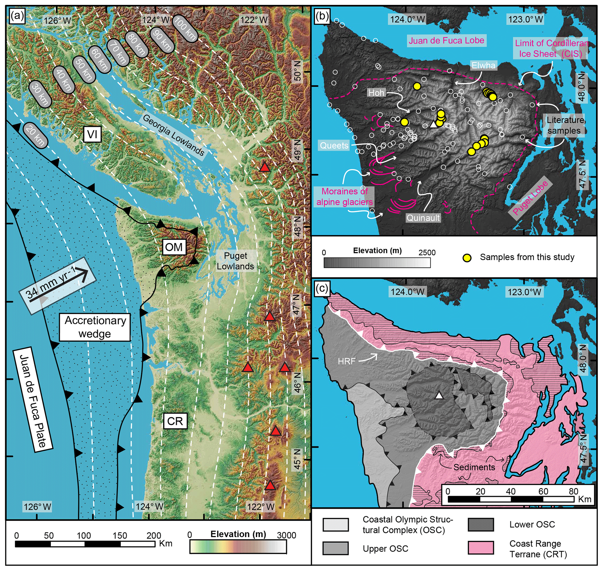
Figure 1(a) Overview map of the Cascadia Subduction Zone showing the extent of the accretionary wedge. White dashed lines are contour lines for the top of the subducted oceanic plate from the Slab1.0 model (Hayes et al., 2012; McCrory et al., 2012), the black arrow indicates the present-day convergence rate and direction at the latitude of the Olympic Mountains (Doubrovine and Tarduno, 2008), and red triangles denote the location of active volcanoes. VI: Vancouver Island, OM: Olympic Mountains, CR: Oregon Coast Range. (b) Topography of the Olympic Mountains, major river valleys (Elwha, Hoh, Quinault, Queets), and major Quaternary features are indicated. Limit of the Cordilleran Ice Sheet from Porter (1964), alpine moraines after geologic map of Tabor and Cady (1978). Locations of samples from this study (filled yellow circles) and previous studies (open white circles) are indicated. The white triangle denotes the location of Mt. Olympus. (c) Geologic and structural map of the Olympic Mountains after Tabor and Cady (1978) and Brandon et al. (1998). The line pattern indicates the occurrence of sediments within the Coast Range Terrane. HRF: Hurricane Ridge Fault.
Based on thermo-kinematic modeling of thermochronometric cooling ages, the Olympic Mountains, USA (Fig. 1a), have been proposed to be in flux steady state since ca. 14 Ma (Batt et al., 2001; Brandon et al., 1998). The approach of these studies was to assume flux steady state along a two-dimensional profile across the Olympic Peninsula as a precondition in order to derive the kinematics of the model from the balance between accretionary influx (governed by the thickness of accreted sediment and plate convergence rate) and denudational outflux (as set by exhumation rates). Because the cooling ages can successfully be modeled with the kinematics used, the mountain range is then interpreted to be in flux steady state. However, possible temporal variations in parameters like sediment thickness, plate convergence rate, or exhumation rates were not considered in these studies. Likewise, the impact of Plio–Pleistocene glaciation on the flux steady-state hypothesis has not been considered yet, although the range was extensively incised by glaciers (Adams and Ehlers, 2017; Montgomery, 2002; Montgomery and Greenberg, 2000; Porter, 1964) and experienced significant changes in climate conditions over the past 3 Myr (Mutz et al., 2018). Numerical modeling studies investigated the mechanics of the wedge by either considering fluvial erosion (Stolar et al., 2007) or glacial erosion (Tomkin and Roe, 2007). A significant response of the orogenic wedge to glaciation was suggested (Tomkin and Roe, 2007) and recent studies proposed that exhumation rates in the Olympic Mountains increased due to Plio–Pleistocene glacial erosion (Herman et al., 2013; Michel et al., 2018). Resulting high sedimentation rates during the Quaternary increased the sediment thickness on the oceanic plate and seem to have caused a change in the deformational style of the offshore part of the wedge (Adam et al., 2004).
In this study, we test the hypothesis of flux steady state in the Olympic Mountains considering variations in both the material influx and outflux. First, we test the temporal steadiness of exhumation rates from bedrock cooling histories with a 1-D thermo-kinematic model, capitalizing on new samples that have been dated with three to four thermochronometers (apatite and zircon (U–Th) ∕ He and fission-track data; AHe, ZHe, AFT, and ZFT, respectively). Second, instead of assuming flux steady state as a precondition, we attempt to estimate both the accretionary influx and denudational outflux independently from each other. We particularly consider possible temporal variations in parameters affecting both fluxes by using published data of the offshore and onshore sediment records and exhumation rates from thermochronometry. With our new thermochronometry data we reveal a previously undetected temporal variation in exhumation rates due to a change in the tectonics (a reduction in plate convergence rates that resulted in a decrease in exhumation rate), as well as the previously reported increase in exhumation rates related to the Plio–Pleistocene glaciation (reflecting a change in climate). Similarly, both material influx and outflux are temporally variable, especially during the Quaternary. A quantitative comparison between the two fluxes suggests that the Olympic Mountains could be in flux steady state over longer timescales (e.g., 107 years) if a three-dimensional geometry is considered.
2.1 Geology and glacial history of the Olympic Mountains
At present, the Juan de Fuca Plate subducts obliquely with respect to the overriding North American Plate (Fig. 1a) at 34 mm yr−1 at the latitude of the Olympic Mountains (Doubrovine and Tarduno, 2008). The forearc high of the subduction zone comprises (from north to south) Vancouver Island, the Olympic Mountains, and the Oregon Coast Range, and it lies west of a forearc low (e.g., Georgia Lowlands, Puget Lowlands) and the active volcanic arc (Fig. 1a). Seismic imaging suggests a flatter subduction angle beneath southern Vancouver Island and the Olympic Mountains (Hayes et al., 2012; McCrory et al., 2012) compared to areas in the north and south (Fig. 1a). The modern configuration of the subduction zone was established by the latest Eocene (e.g., Brandon and Vance, 1992) after accretion of the Coast Range Terrane to the North American continent (Fig. 1c). This terrane represents a large oceanic plateau and extends from the southern tip of Vancouver Island to Oregon (Eddy et al., 2017; Phillips et al., 2017; Wells et al., 2014).
The accretionary wedge of the subduction zone is exposed onshore within the Olympic Mountains (Fig. 1a) and is composed of Eocene–Miocene flysch (Brandon et al., 1998; Tabor and Cady, 1978). This part of the mountain range is known as the Olympic Structural Complex (Brandon et al., 1998) and is separated from the surrounding Coast Range Terrane by the Hurricane Ridge thrust fault (HRF; Fig. 1c), a major discontinuity traceable in seismic surveys (e.g., Clowes et al., 1987; Calvert et al., 2011). Minor sedimentary rocks of Eocene age (Eddy et al., 2017; Tabor and Cady, 1978) are contained within the Coast Range Terrane besides the predominant ∼50 Ma marine and subaerial basaltic rocks (Eddy et al., 2017). Exhumation of the range commenced at 18 Ma and since 14 Ma, the orogen is presumed to be in flux steady state (Batt et al., 2001; Brandon et al., 1998; Pazzaglia and Brandon, 2001).
Plio–Pleistocene glaciation has strongly influenced the present-day appearance of the Olympic Mountains (Fig. 1b). During its maximum extent at ∼14 ka, the Cordilleran Ice Sheet advanced from the Coast Mountains of British Columbia and covered Vancouver Island and large parts of the current continental shelf (Booth et al., 2003; Clague and James, 2002). The Puget and Juan de Fuca lobes of the Cordilleran Ice Sheet surrounded the Olympic Mountains in the east-southeast and in the north, respectively (Fig. 1b). Alpine glaciers incised deep valleys in the landscape, particularly on the western side of the range (Adams and Ehlers, 2017; Montgomery, 2002), where piedmont glaciers almost reached the Pacific Ocean (Thackray, 2001). Glacial erosion varied across the range, as the location of the Pleistocene equilibrium line altitude increases from 1000 m in the west to 1800 m in the east (Porter, 1964) due to a strong precipitation gradient (> 6000 mm yr−1 in the west, < 1000 mm yr−1 in the east). Determining the exact onset of glaciation in the Olympics has proven difficult, but the oldest deposits of the Cordilleran Ice Sheet in the Puget Lowland are as old as 2 Ma and deeply weathered alpine till on the west side of the Olympics is interpreted to be of the same age (Easterbrook, 1986).

Figure 2Map of new and previously published thermochronometric ages within the Olympic Mountains for (a) AHe, (b) AFT, (c) ZHe, and (d) ZFT. Data from the literature (Batt et al., 2001; Brandon et al., 1998; Brandon and Vance, 1992; Michel et al., 2018; Stewart and Brandon, 2004) are indicated by circles with a black dot. Note that the color coding of the symbols varies between panels. For AFT literature samples, the different reset states (fully reset, incompletely reset, and unreset) are indicated by symbol shape. Maps of exhumation rates as suggested by (e) Michel et al. (2018) and (f) Brandon et al. (1998). The white triangle denotes the location of Mt. Olympus.
2.2 Previous thermochronometry studies in the Olympic Mountains
Within the Olympic Mountains, there is an extensive dataset of thermochronometric cooling ages from bedrock samples (Figs. 1b and 2) for AHe (Batt et al., 2001; Michel et al., 2018), AFT (Brandon et al., 1998), ZHe (Michel et al., 2018), and ZFT (Brandon and Vance, 1992; Stewart and Brandon, 2004). These thermochronometer systems record cooling through a temperature range of ∼60–240 ∘C (e.g., Brandon et al., 1998; Farley, 2002; Gallagher et al., 1998; Reiners et al., 2004), as they have effective closure temperatures of 70, ∼120, ∼180, and ∼240 ∘C, respectively, for a cooling rate of ∼10 ∘C Myr−1 (Ehlers, 2005). The interpretation of thermochronometric cooling ages from sedimentary rocks (such as in the Olympic Mountains) is often complicated when the cooling signal from the sediment source region(s) has not been reset due to reheating during subduction and metamorphism. If a sedimentary rock sample has not had sufficient exposure to temperatures above the closure temperature of a given thermochronometer, the sample might retain cooling ages that represent the source region's cooling history (referred to as unreset) or might be a mixture of provenance cooling histories and the reheating process (incompletely reset sample). Determining whether a sample is completely reset, incompletely reset, or unreset can be difficult and usually depends on the statistics of cooling age populations derived from the dated mineral grains (e.g., Brandon et al., 1998). The reproducibility of single-grain (U–Th) ∕ He ages from a sample provides an indication of whether a sample is reset or not. This is typically determined with n=4–7 grains. For the fission-track method, a larger number of grains is typically dated (n=20–100) to reduce the uncertainty in the final cooling age calculation. For samples with a large population, statistical methods can be applied to decompose the chronometer date distribution into different populations and to determine if some portion of the sample is reset (Brandon, 1992, 1996). In the case in which a sample is incompletely reset, a significant young age peak is determined and interpreted as the sample cooling age (e.g., Brandon et al., 1998).
In the Olympics, the youngest published reset AHe ages (≤2.5 Ma) can be found in the western and central portions of the mountain range, and there are two unreset samples in the east (Fig. 2a). The pattern of AFT ages is more complicated (Fig. 2b), and most reset and incompletely reset samples are located in the central part of the mountain range, whereas unreset samples are restricted to areas outside the central (high-topography) part of the range. The youngest reported AFT samples (2–4 Ma) are incompletely reset samples, and fully reset samples have cooling ages between 7 Ma and 27 Ma. ZHe data show a well-developed trend of unreset cooling ages at the coast and reset 5–6 Ma ages in the headwaters of the Hoh and Elwha rivers (compare Figs. 1b and 2c). Reset ZFT samples (∼13–14 Ma) are confined to a small area east of Mt. Olympus (Fig. 2d).
Based on thermo-kinematic modeling, Michel et al. (2018) attributed the observed AHe and ZHe age pattern to an ellipse-shaped exhumation pattern (with highest exhumation rates in the central, high-topography part of the mountain range; Fig. 2e), as predicted for a mountain range situated in an orogenic syntaxis setting (Bendick and Ehlers, 2014). Here, a bend in the subducted slab creates a mechanical stiffening, which in turn leads to rapid and focused exhumation at the surface (Bendick and Ehlers, 2014). High uplift rates in the central, high-topography part of the mountain range are also corroborated by topographic analyses (Adams and Ehlers, 2017) and denudation rates based on cosmogenic nuclides (Adams and Ehlers, 2018). Furthermore, modeling of particularly young AHe ages (< 2.5 Ma) suggests that exhumation rates increased significantly by 50 %–150 % due to Plio–Pleistocene glacial erosion (Michel et al., 2018).
Table 1Data for the ocean drill cores shown in Fig. 3.
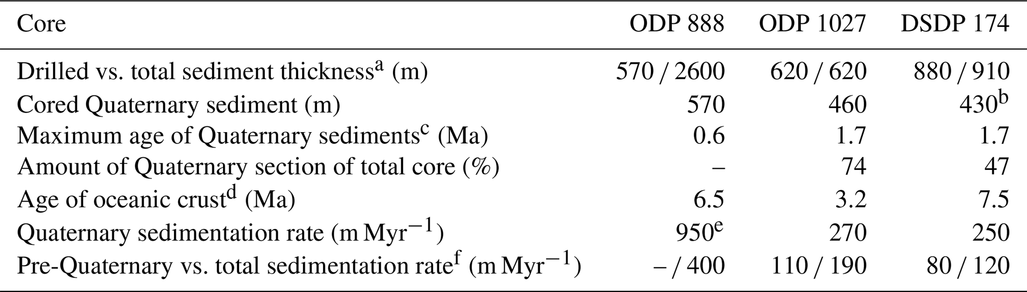
For core ODP 888, information is taken from Westbrook et al. (1994), for ODP 1027 from Su et al. (2000), and for DSDP 174 from Kulm et al. (1973). Sedimentation rates are calculated in this study using the reported thicknesses and age constraints. a If total thickness exceeds drilled thickness, then the total thickness was estimated from seismic data (e.g., ODP 888). b Due to poor core recovery, the Plio–Pleistocene boundary can only be confined between 418 and 446 m. c Ages based on biostratigraphy. For cores ODP 1027 and DSDP 174, the Plio–Pleistocene boundary was recovered and an age of 1.7 Ma is used here as reported by Su et al. (2000). d For cores ODP 888 and DSDP 174, the age refers to the age of the oceanic crust and is taken from Fig. 3 at the respective location of the core. For ODP 1027, the age refers to the age of the oldest sediment in the core taken from Su et al. (2000). e This rate is calculated for the recovered core interval, which only encompasses 600 kyr. f The total sedimentation rate equals the total thickness divided by the age of the oceanic crust.
2.3 Offshore sediment record
Data constraining the sediment thickness on the Juan de Fuca Plate before the incorporation of sediment into the accretionary wedge are summarized in Fig. 3. Three boreholes were drilled into the blanketing sediments of the Juan de Fuca Plate during deep-sea drilling projects (ODP 888, ODP 1027, and DSDP 174; Fig. 3 and Table 1) and provide estimates of the sediment thickness and age constraints. The sediment thickness at the deformation front of the subduction zone has been estimated from three seismic studies (Adam et al., 2004; Booth-Rea et al., 2008; Han et al., 2016).
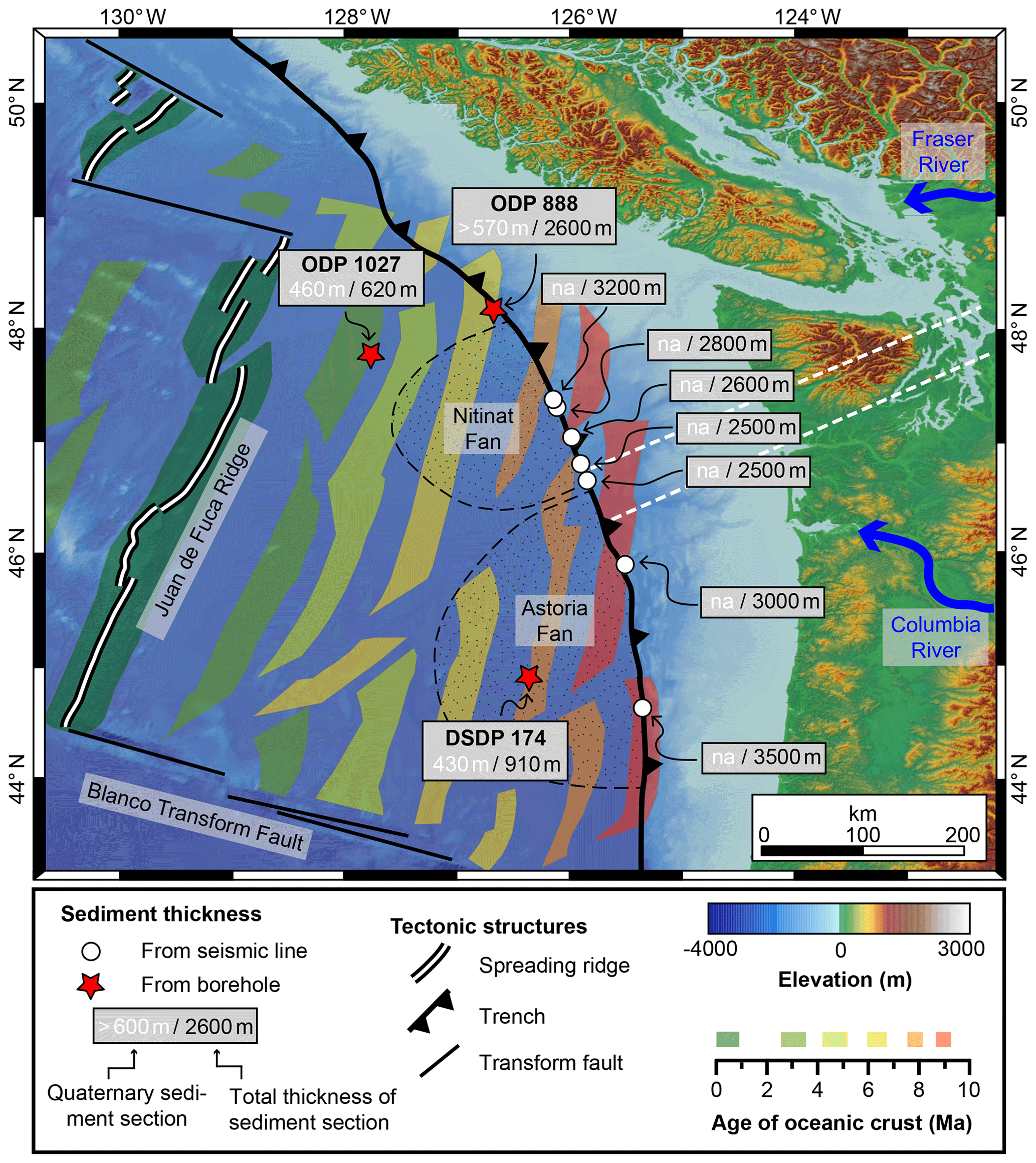
Figure 3Map of the Cascadia Subduction Zone showing the age of the oceanic crust (Wilson, 1993) and sediment thickness, estimated from the sediment cores of ocean drilling programs (holes ODP 888, OPD 1027, and DSDP 174) and seismic studies (Adam et al., 2004; Booth-Rea et al., 2008; Han et al., 2016). The amount of Quaternary sediment material estimated from cores is also included (Kulm et al., 1973; Su et al., 2000; Westbrook et al., 1994); more information about the drill cores is provided in Table 1. The locations of two major submarine fans (Nitinat Fan and Astoria Fan) are indicated by the dotted pattern. The Fraser and Columbia rivers are the main modern sediment sources for the Nitinat and Astoria fans, respectively. White dashed lines indicate the position of cross sections presented in this study (see also Fig. 7).
Most of the sediment is contained within two deep-sea sediment fans with different sediment sources. Today, sediment sources for the Nitinat Fan (offshore of Vancouver Island and the Olympic Mountains) include detritus from Vancouver Island, the Olympic Mountains, and material delivered by the Fraser River system (Fig. 3), which drains large parts of the Canadian Cordillera including the British Columbian Coast Mountains (Carpentier et al., 2014; Kiyokawa and Yokoyama, 2009). The Astoria Fan offshore of the Oregon coast is mostly fed by the Columbia River and is sourced by a large area in the interior of the USA (Fig. 3).
The total sediment thickness varies between 2600 and 3500 m at the deformation front and decreases rapidly to 600 or 900 m approximately 100 km away from the deformation front. At the locations of ODP 1027 and DSDP 174, up to 50 %–70 % of the total sediment thickness is made up of Quaternary deposits, and sedimentation rates more than doubled during the Quaternary (from 80–110 to 250–270 m Myr−1; Table 1). At the location of ODP 888 the drilled 570 m of core was deposited over the past 600 kyr, suggesting very high sedimentation rates of 950 m Myr−1 compared to 400 m Myr−1 for the total sediment thickness of 2600 m at the location of the core (Table 1). As determined from a detailed stratigraphic analysis of core ODP 888, sedimentation rates are also highly variable during the Quaternary. Rates during glacial periods can be as high as 1900 m Myr−1 compared to 700 m Myr−1 during interglacials (Knudson and Hendy, 2009). At sites ODP 888 and 1027, the source region of the sediments has been the Canadian Cordillera for the past 3.5 Myr, which has not been affected by glacial–interglacial cycles (Carpentier et al., 2014; Kiyokawa and Yokoyama, 2009). The provenance of the sediments at DSDP 174 is mostly the Proterozoic Belt Supergroup in the interior of the USA and differs significantly from present-day detritus of the Columbia River (Prytulak et al., 2006). Hence, Prytulak et al. (2006) suggest that the deposition of the upper 630 m of sediment at this site and the buildup of the Astoria Fan were governed by glacial outburst floods.
We use a multi-method approach to assess flux steady state in the Olympic Mountains. This includes thermochronometric dating, thermo-kinematic modeling of cooling ages to obtain exhumation rates, and independent estimates of accretionary influx and denudational outflux. We calculate the influx based on constraints of the incoming sediment thickness and plate convergence rate and the outflux based on spatial constraints of exhumation rates within the Olympic Mountains. The procedure for each method is outlined below.
Table 2Coordinates, elevations, and thermochronometric cooling ages for samples considered in this study.

Samples in italics are used for 1-D thermo-kinematic modeling. Results from single-grain analyses for AHe and ZHe are reported in Tables S1 and S2, respectively. Further details for AFT and ZFT dating can be found in Table 3, and single-grain analyses for apatite and zircon are reported in Tables S3 and S4, respectively. 1 SD indicates 1 standard deviation, nd: not determined. a AHe and ZHe ages of the respective samples are from Michel et al. (2018). b Reported sample AHe ages are single-grain ages because the yield of suitable apatite grains did not allow us to date more grains.
3.1 Thermochronometric methods
Our strategy with thermochronometric dating was (1) to obtain samples that are multi-dated with up to four thermochronometer systems (because these are particularly sensitive to reveal variations in exhumation rate) and (2) to collect samples within vertical profiles in order to obtain estimates of the exhumation rate at the site of the respective profile. Therefore, we dated several literature samples with additional thermochronometer systems (Table 2) and we also present 19 new bedrock samples from vertical profiles (Fig. 4, Table 2) and two additional bedrock samples (OP1528 and OP1556; Fig. 2, Table 2) collected at an elevation of ∼400 m, enlarging the existing ∼400 m equal-elevation data of Michel et al. (2018). All new samples are sandstones of varying grain size. A sample transect at Mt. Olympus extends from the bottom of the Hoh Valley to the apex of the Olympic Peninsula (Mt. Olympus, 2428 m), covering ∼2 km of relief (Fig. 4a and b). The Mt. Anderson transect starts in the upper reaches of the Quinault Valley and terminates on the flank of Mt. Anderson, covering a total elevation difference of ∼1600 m (Fig. 4a and c). The Blue Mountain transect is located in the northern part of the Olympic Peninsula close to Blue Mountain, covering an elevation difference of ∼1300 m (Fig. 4a and d). All collected samples were dated with the AHe and ZHe techniques; three were dated by AFT, and two were dated by the ZFT technique. Additionally, we dated 13 samples from Michel et al. (2018) by AFT and 5 by ZFT thermochronometry. This process yielded seven samples with AHe, AFT, ZHe, and ZFT cooling ages (Table 2).
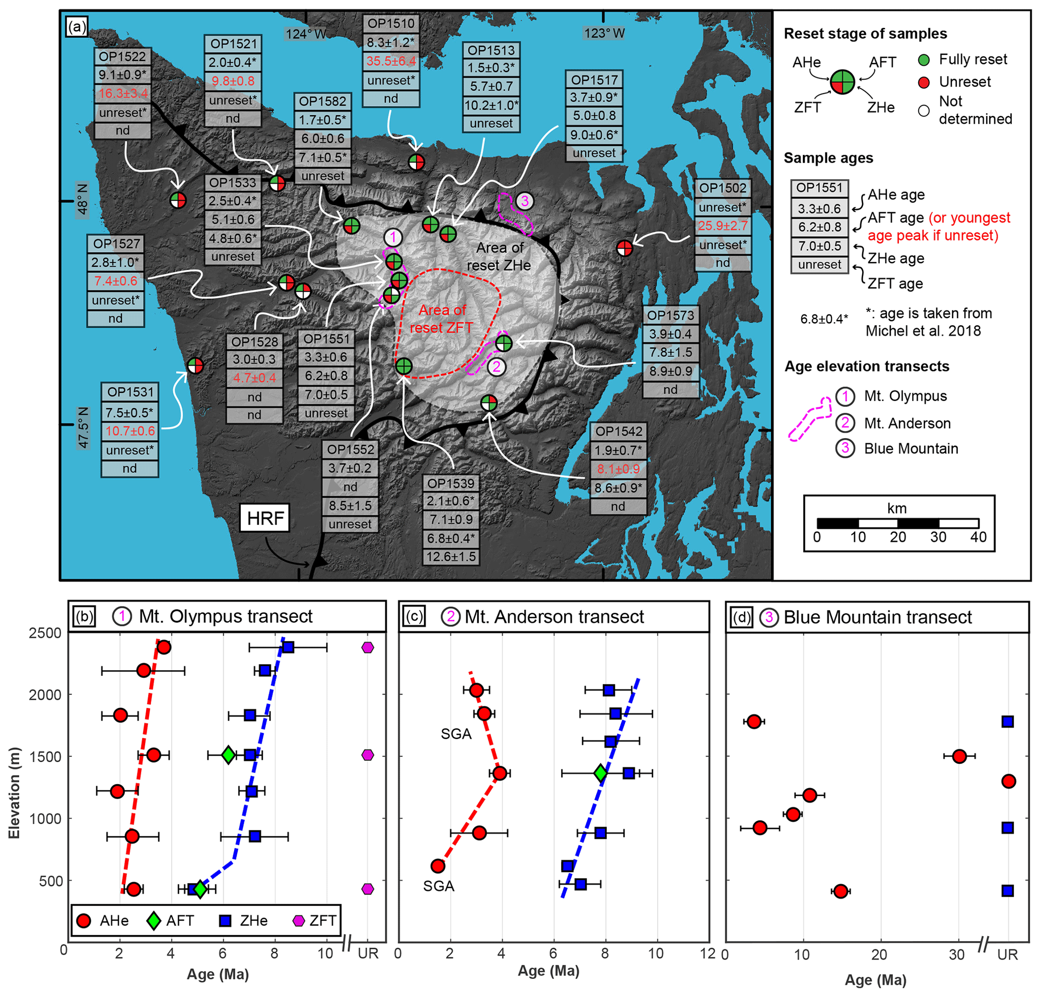
Figure 4(a) Map of samples for which three to four different thermochronometer systems are available. The pie charts show the reset stage of a particular thermochronometer system for the sample. If AFT ages are unreset, the peak age of the youngest age population is given as the sample age (see Table 3 for older populations). Ages denoted with an asterisk are taken from Michel et al. (2018). The Hurricane Ridge Fault (HRF) separates the rocks of the accretionary wedge from the surrounding Coast Range Terrane in the hanging wall. The locations of the three different elevation transects (Mt. Olympus, Mt. Anderson, and Blue Mountain) are indicated on the map and the resulting age–elevation plots are shown in (b) to (d). In (b) and (c) the dashed colored lines correspond to possible exhumation rates interpreted from the respective thermochronometer. All uncertainties are 1 standard deviation, SGA: single-grain age.
Standard mineral separation techniques (sieving, magnetic and gravimetric separation) were used to obtain apatite and zircon separates from crushed rock samples. For AHe and ZHe dating mineral grains were handpicked and dated in the thermochronometry lab of the University of Tübingen, following the dating protocol of Stübner et al. (2016). The Ft correction for apatite (Farley, 2002) and zircon (Hourigan et al., 2005) is applied to the measured amount of helium. The (U–Th) ∕ He age equation is solved using the approach of Meesters and Dunai (2005). From each sample, we dated four to seven apatite grains or three to six zircon grains and the results of single-grain analyses can be found in Tables S1 and S2 in the Supplement. Our approach for assessing whether a sample is reset or unreset and the procedure for the exclusion of outliers are explained in the Supplement (Sect. S1.1). For reset samples, we calculate the arithmetic mean age from the accepted single-grain ages, which is reported in Table 2 along with a 1 standard deviation (1 SD) uncertainty.
Table 3Results from fission-track dating.
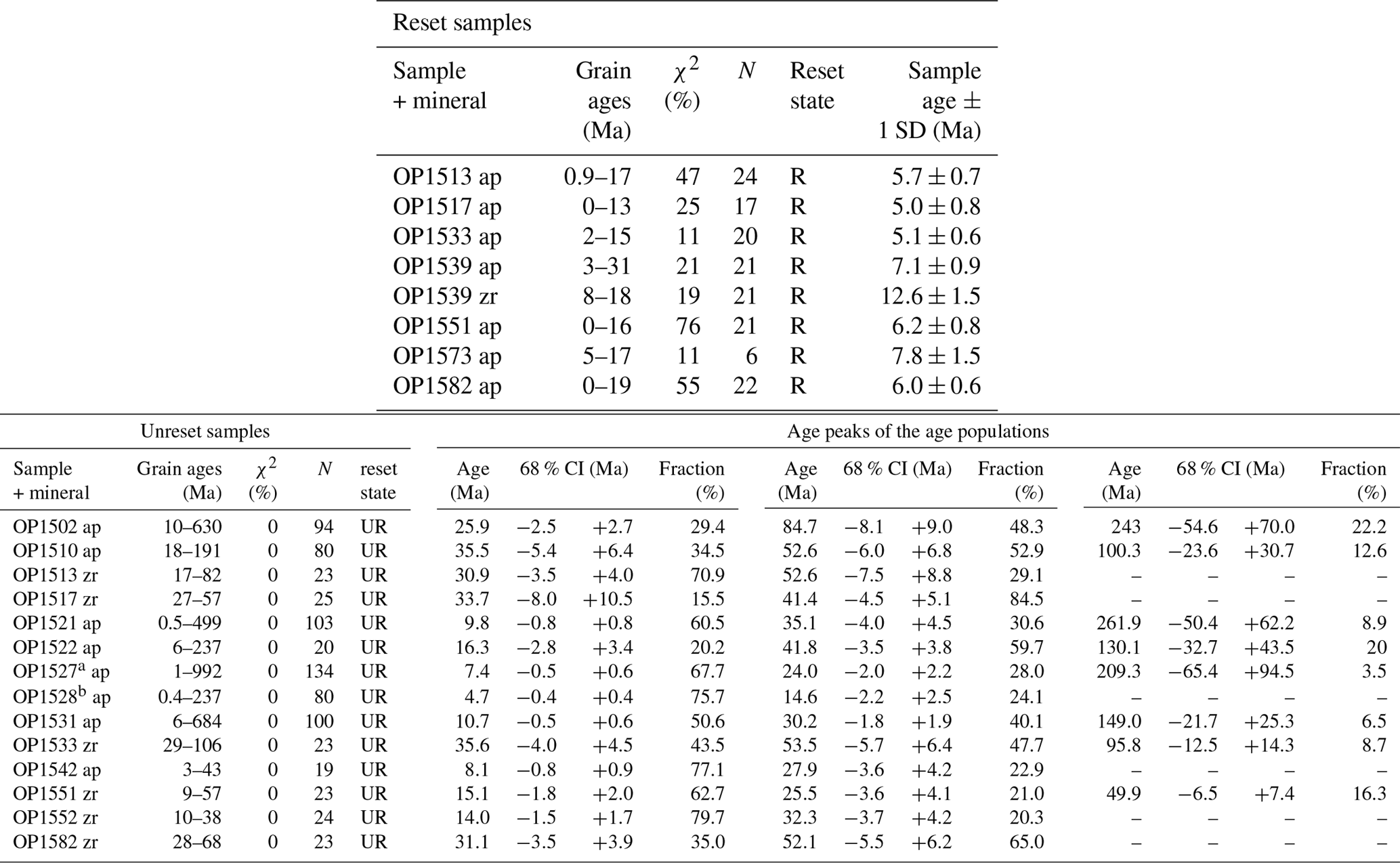
For AFT and ZFT, 20 grains per sample were dated in a first step and it was checked whether the sample passes the χ2 test and can be considered as reset (i.e., >5 %; an indication of belonging to the same age population; e.g., Galbraith, 2005). If so, the pooled ζ age was considered as the sample age and reported here. If a sample failed the χ2 test (i.e., <5 %), the sample is considered unreset and, in the case of AFT, 100 grains were dated if enough grains were available. The detrital age distribution was then decomposed into detrital age populations using BINOMFIT (Brandon, 1992, 1996) and the peak ages of those populations (with asymmetric error range for each age peak corresponding to the 68 % confidence interval; CI) are reported. For the ZFT method, information on whether the sample is reset or unreset is sufficient for this study and no further grains were dated. “Fraction” equals the number of grains contained within the respective age peak. N is the number of counted grains. Contrary to Brandon et al. (1998), we did not consider multiply or partially reset AFT samples but treated them as unreset because our thermo-kinematic model can only be applied to fully reset samples. a Results for this sample are obtained by merging grains from our sample OP1527 (n=103) and sample AR39 (n=31) from Brandon et al. (1998). b Results for this sample are obtained by merging grains from our sample OP1528 (n=68) and sample AR40 (n=12) from Brandon et al. (1998).
Fission-track dating of apatite and zircon was performed using an external detector and ζ-calibration techniques (Hurford, 1990). Details about the treatment of the apatite and zircon mounts in the Tübingen thermochronometry laboratory can be found in Falkowski et al. (2014) and Falkowski and Enkelmann (2016). Table 3 contains the AFT and ZFT sample ages and explains the procedure for assessing whether a sample is reset or unreset. Data for single-grain ages from fission-track dating of apatite and zircon are reported in Tables S3 and S4.
3.2 Thermo-kinematic modeling: model setup and boundary conditions
To interpret cooling histories recorded by our thermochronometers as exhumation histories, we used a modified version of the thermo-kinematic model Pecube (Braun, 2003), which contains a built-in Monte Carlo approach to resolve temporal variations in exhumation histories (Adams et al., 2015; Thiede and Ehlers, 2013). The model allows for the exploration of possible exhumation histories for a particular sample by varying exhumation rates through time at defined time steps. The accuracy of a particular exhumation rate history is estimated by comparing modeled with observed cooling ages. More age constraints, and hence thermochronometer systems, lead to better-resolved modeled exhumation histories. Therefore, although we report 21 new thermochronometric ages, we only used the seven samples that have age constraints from AHe, AFT, ZHe, and ZFT in our modeling efforts (OP1513, OP1517, OP1533, OP1539, OP1551, OP1573, OP1582; Table 2).
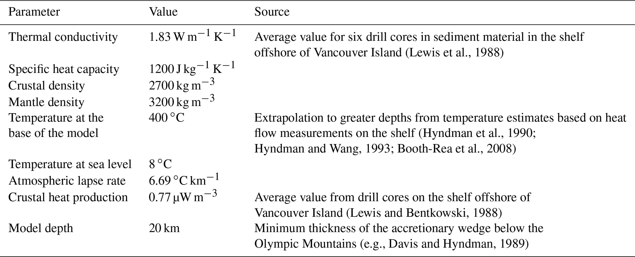
The thermophysical parameters chosen for the modeling are typical values reported for the sandstones of the Olympic Mountains (Table 4). We performed a sensitivity analysis in order to find the most suitable time step for our simulations and the results of that analysis can be found in the Supplement (Sect. S2). Based on the analysis, a time step interval of 1 Myr seems to be most appropriate to use, given the range of our thermochronometry ages and their respective uncertainties. During further modeling, we initiated the models at 20 Ma and used the time step interval of 1 Myr with a maximum testable exhumation rate of 6 km Myr−1. For each sample, we ran 20 000 simulations (each corresponding to a different exhumation history) and assessed the goodness of fit between observed and modeled data for the respective exhumation history using a reduced χ2 test. Here, sample ages τo were compared with modeled ages τm using the uncertainty of the sample age σo for the number (N) of thermochronometer systems available for the respective sample:
If χ2≤2, a specific model run was accepted as good. The number of accepted exhumation histories is shown in Fig. 5 for each sample. From the range of acceptable exhumation rates at each time step (shown as blue shaded areas in Fig. 5), we calculated the mean exhumation rate together with 1 standard deviation for each time step (red dashed lines and grey areas in Fig. 5). Although the model provides output for the entire model duration of 20 Myr, a meaningful exhumation rate can only be obtained for the time interval between the oldest thermochronometric age of a sample and today (shown in Fig. 5).

Figure 5Results from thermo-kinematic Monte Carlo modeling for the seven considered samples (OP1513, OP1517, OP1533, OP1539, OP1551, OP1573, OP1582). The location of each sample within the Olympic Peninsula is shown, together with the respective elevation (Elev). The entire range of exhumation rates from the number of accepted model runs (N) is outlined by the blue shaded area, from which the mean rate and 1 standard deviation (1 SD) is calculated at each time step. Black, green, and blue stippled boxes outline measured AHe, AFT, and ZHe ages of the samples with 1 SD.
For our purpose, we focus on exploring temporal variations in exhumation rates and therefore use a 1-D model, whereby each sample is modeled independently from each other. In a 1-D model, heat transport and the movement of particles are only considered in the vertical dimension within a column of rock, ignoring topography. This mode of modeling was selected because it allowed us to efficiently perform thousands of simulations quickly in order to cover a large range of possible exhumation rates. The high number of exhumation histories accurately predicts our observed cooling ages and allows for a robust statistical assessment of the best-fitting exhumation history. Previous publications addressing exhumation histories in other orogens have also highlighted the fact that 1-D models are often sufficient to explain most of the signal recorded in thermochronometric systems (e.g., Adams et al., 2015; Thiede and Ehlers, 2013). In the Olympic Mountains, Michel et al. (2018) argued that exhumation histories for the thermochronometer systems considered here can also be explained well by vertical velocity paths. Because the spatial resolution of our seven considered samples is poor and they are all from the interior part of the mountain range (Fig. 4), we cannot further resolve the exhumation rates outside this area, making a 3-D model very difficult to validate. Therefore, we limit our interpretations to the better-resolved exhumation histories from the 1-D model and focus on the primary temporal changes, rather than paleotopography, or specific differences in the exhumation rates between samples.
Five of the seven considered samples are from the same elevation range (400–580 m), but two samples are from higher elevations (1360 and 1500 m; Fig. 5). Large differences in elevation between the samples can impact the direct comparison between them (e.g., it can affect how changes in exhumation rate are recorded from location to location). However, we are not able to correct for this circumstance (by using an age–elevation relationship) and therefore try to consider this complication when interpreting our exhumation rate histories from the different samples.
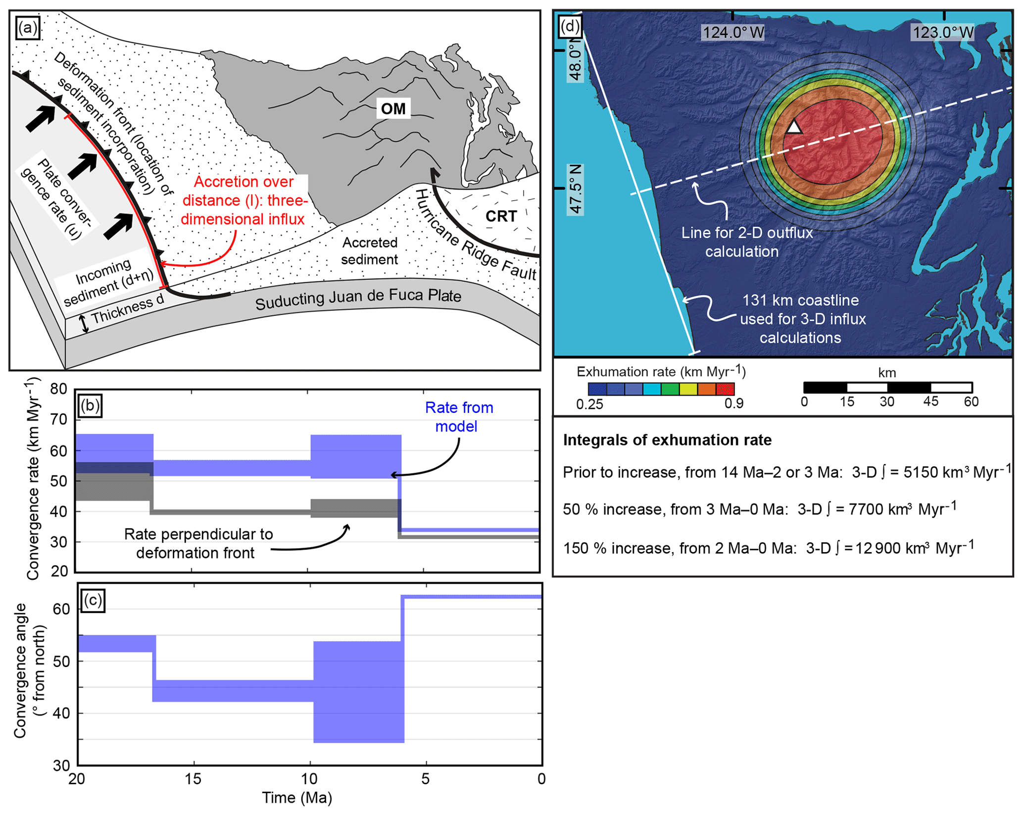
Figure 6Constraints used for our quantitative accretionary influx and denudational outflux calculations. (a) Cartoon illustrating our approach for calculating the accretionary influx. The influx corresponds to the sediment scraped off the subducting Juan de Fuca Plate and is governed by the plate convergence rate (u) and the incoming sediment properties (thickness d, porosity η). Because we use a three-dimensional geometry, accretion is considered along a length (l) within a vertical plane. This length corresponds to the length of the coastline indicated in panel (d). OM: Olympic Mountains, CRT: Coast Range Terrane. After Batt and Brandon (2002). (b) Temporal evolution of the plate convergence rate used in the calculations, considering only the component perpendicular to the deformation front (black envelope), and the original output (blue envelope) from the plate reconstruction model of Doubrovine and Tarduno (2008). To provide an uncertainty for our calculations, we consider a range of convergence rates (comprising the width of the envelope) for each time step based on two different rotation models in the model of Doubrovine and Tarduno (2008) (see text for details). (c) Temporal evolution of the plate convergence angle (Doubrovine and Tarduno, 2008) used to correct the plate convergence rate in (b). (d) Exhumation rate pattern from Michel et al. (2018) used for our outflux calculations. The range of displayed rates (0.25–0.9 km Myr−1) corresponds to the rates prior to the glacially induced increase in exhumation rates. The outflux is based on the spatial integration of the exhumation rate pattern. Values for the integrals are listed below the plot for the respective increase in exhumation and time. The white dashed line was used for integrating the exhumation rate using a two-dimensional geometry, which is further explained in the Appendix.
3.3 Methods for estimating flux steady state
To assess the flux steady-state hypothesis of the Olympic Mountains, we need independent estimates of the material influx and outflux over time. For this, we focus on the time period since 14 Ma, which corresponds to the proposed establishment of flux steady state (Batt et al., 2001; Brandon et al., 1998). Flux steady state requires that the material influx into the wedge equates to the amount of accreted material removed from the subducting slab. We assessed the amount of accreted sediment (material influx) with two approaches. First, we calculated the amount of sediment incorporated into the accretionary wedge at the deformation front (Fig. 6a) during the 14 Myr period. Second, we compared this amount of “expected” accreted sediment with the observed amount of sediment residing in the accretionary wedge along two cross sections. The material outflux from the mountain range is estimated using results from thermo-kinematic modeling by equating modeled exhumation with denudation, which can then be integrated spatially and over the 14 Myr period.
Previous flux steady-state analyses in the Olympic Mountains were performed in two dimensions along a profile crossing the Olympic Peninsula. However, exhumation rates within the Olympic Mountains are known to vary spatially (Brandon et al., 1998; Michel et al., 2018). This suggests that the outflux is spatially variable, depending on the location within the mountain range. Hence, we performed our flux analysis in three dimensions and the resulting geometries are summarized in Fig. 6. The influx is calculated along the length of the deformation front, and for the calculation of the outflux we considered almost the entire area of the Olympic Peninsula.
3.3.1 Calculating the accretionary influx
We used a similar approach as Batt et al. (2001) to calculate the accretionary influx, but used a three-dimensional geometry and additionally considered temporal variations in the variables used. Assuming all sediments resting on the subducting oceanic crust are incorporated into the accretionary wedge, the volume of accreted sediment (Vsed) can be approximated using the porosity of the sediment η, incoming sediment thickness d, length of the coast l, the duration of subduction t, and the subduction velocity perpendicular to the present-day deformation front uper:
A limitation to this approach is the assumption that all sediment resting on the down-going plate is accreted. There is geochemical evidence that, at early stages of subduction at the Cascadia Subduction Zone, sediment has been incorporated into the mantle and was involved in the magmatism of the Cascades Arc (Leeman et al., 2005; Mullen et al., 2017). However, there are no estimates on the amount of sediment transported into the mantle at present, and most sediments seem to be accreted either at the deformation front or underplated at depth (Calvert et al., 2011).
Table 5Results from influx and outflux calculations using a three-dimensional geometry.
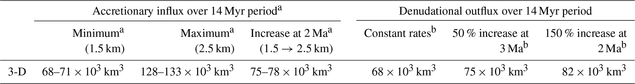
The entire procedure for calculating the influx and outflux is described in Sect. 3.3. The influx volumes are reported as ranges because minimum and maximum convergence rates (Fig. 6b) have been obtained from the plate reconstruction model of Doubrovine and Tarduno (2008). a Sensitivity to incoming sediment thickness: the accretionary influx volume is calculated for three different sediment thicknesses, yielding a minimum volume (1.5 km thickness), maximum volume (2.5 km thickness), and a more realistic volume (whereby the volume increases from 1.5 to 2.5 km at 2 Ma). b Sensitivity to an increase in exhumation rates: the denudational outflux volume is calculated assuming constant exhumation rates and considering the increase in exhumation rates due to glacial erosion, with an increase by 50 % at 3 Ma or an increase by 150 % at 2 Ma. Exhumation rates are based on Michel et al. (2018) and displayed in Fig. 6d and e.
The variable with the greatest uncertainty in this calculation is the sediment thickness back in time that has now been subducted below the Olympic Mountains. As discussed above (Sect. 2.3), the present-day sediment thickness of 2.5 km is the product of increased offshore sedimentation during the Quaternary, and the pre-Quaternary sediment thickness is difficult to determine. Following the approach described in the Supplement (Sect. S3.1), we estimated a pre-Quaternary sediment thickness of 1.5 km. In total, we calculated three different sediment volumes based on different sediment thicknesses (Table 5). Assuming a thickness of 1.5 and 2.5 km for the 14 Myr period yields a minimum and maximum value for the accreted sediment volume, respectively, representing a sediment volume unaffected by Quaternary sedimentation (1.5 km) and a volume for a likely too-high sediment thickness, using the modern thickness (2.5 km). Alternatively, we considered an increase in sediment thickness from 1.5 to 2.5 km at 2 Ma, which likely yields the geologically most meaningful volume.
The porosity of the sediment stack depends on the thickness and decreases with increasing overburden. According to Yuan et al. (1994), the porosity at depth z of the sediment stack can be approximated by
Using this equation, we calculated mean porosities of 31 % and 22 % for our sediment thicknesses of 1.5 and 2.5 km, respectively.
Because the dip direction of the present-day deformation front is 72∘ (Φdef) and we only considered accretion perpendicular to the deformation front, we corrected the convergence rate (u) by using the convergence angle (Φ) between the Juan de Fuca and the North American plates:
Both the convergence rate and angle are variable over time, and therefore we capitalized on the plate reconstruction model of Doubrovine and Tarduno (2008) to estimate these parameters over the past 14 Myr. Values shown in Fig. 6b and c were calculated using the East–West Antarctica plate circuit model from Doubrovine and Tarduno (2008) for two different rotation models (Farallon M1 and M2 in the original publication). This yields a range of possible convergence rates and angles, providing an uncertainty on the calculated sediment volume. The temporal resolution is given by the number of magnetic isochrons used for the plate circuit reconstruction by Doubrovine and Tarduno (2008). From the temporal evolution of the corrected convergence rate (Fig. 6b), we calculated the sediment volume Vsed accreted during the 14 Myr period using Eq. (2) and the parameters discussed above. For the length l in Eq. (2) we assumed a value of 131 km, which corresponds to the length of the coastline in the area of the exhumation rate pattern (Fig. 6d). The calculated sediment volumes are reported in Table 5.
3.3.2 Sediment volumes along cross sections
We estimated the actual volume of sediment currently residing in the accretionary wedge along two cross sections, which are approximately 50 km apart (Profile 1 and 2 in Fig. 7). The lower boundary of the accretionary wedge is the top of the subducting oceanic plate, which is constrained from the Slab 1.0 model (Hayes et al., 2012; McCrory et al., 2012). The upper boundary is defined by the present-day topography and bathymetry (from 10 and 500 m resolution digital elevation models, respectively) and the Hurricane Ridge Fault (HRF). At the surface, the location of the HRF is adopted from a geologic map (Tabor and Cady, 1978) and below the surface we use information provided by a seismic study at depths of 22 and 34 km (Calvert et al., 2011). The uncertainty related to the position of the HRF (error bars at HRF nodes in Fig. 7) was propagated to estimate an uncertainty for the calculated sediment volumes. A further explanation of this approach is given in the Supplement (Sect. S3.2). Because the location of the HRF is not resolved at greater depths, we truncate the area considered for volume calculation at 34 km of depth. Finally, the calculated volume is corrected for the porosity of the sediment stack. Davis and Hyndman (1989) use porosities of 4 %–10 % for sediments contained within the accretionary wedge offshore of Vancouver Island. Hence, we use an average porosity of 6 % in our correction.
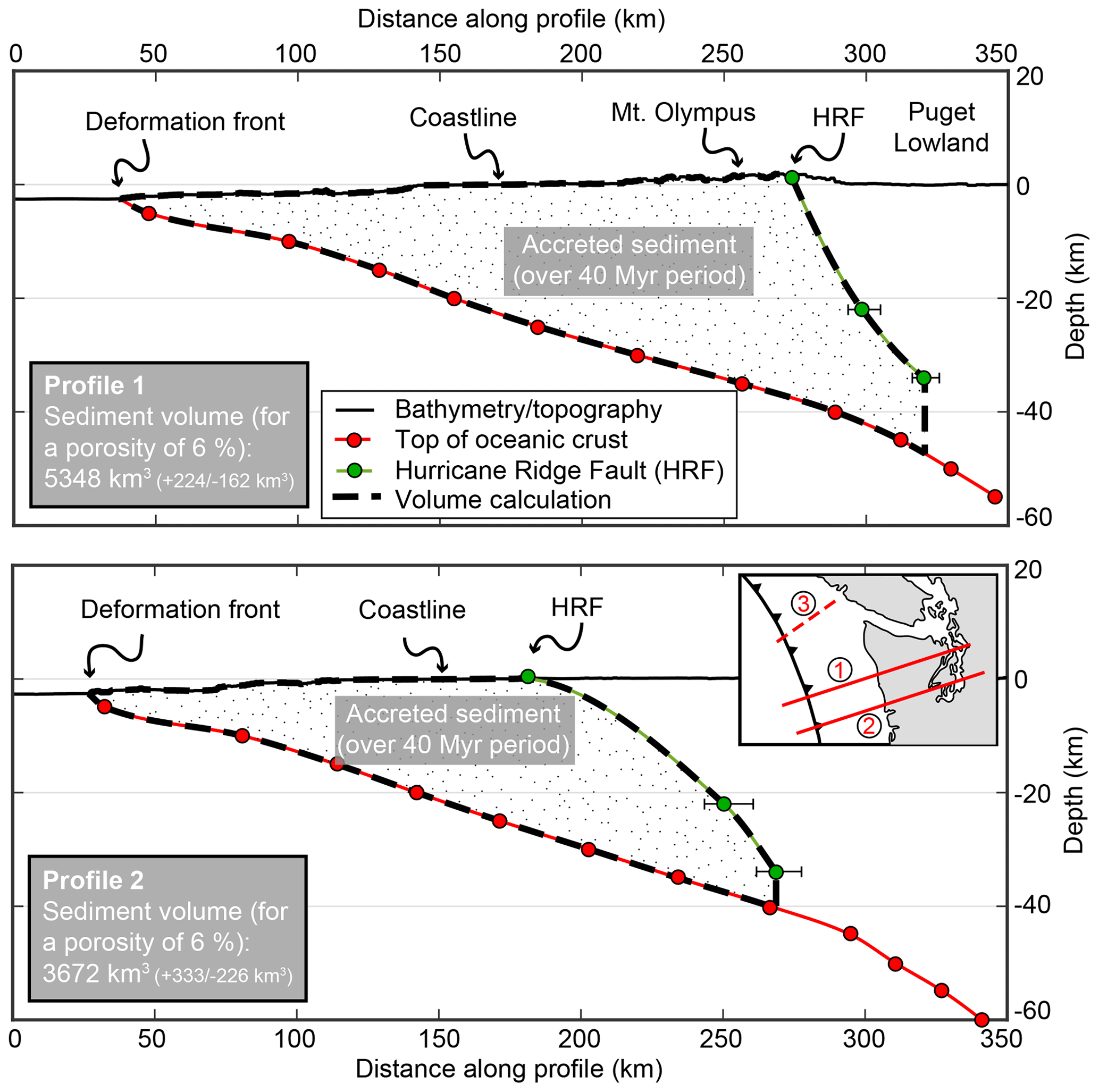
Figure 7Sediment volumes calculated along two cross sections spanning the Olympic Peninsula (Profile 1 and 2, the vertical exaggeration is 2; see inset for location). For an explanation of the procedure used, see the text. The reported uncertainties for the volume are based on the uncertainties in the position of the Hurricane Ridge Fault (indicated with error bars at the respective symbol). Numbers in the inset correspond to the following: (1) position of Profile 1, (2) position of Profile 2, and (3) position of profile by Davis and Hyndman (1989) referred to in the text.
3.3.3 Calculating the denudational outflux
In the absence of extensional faults, denudation acts as the prime mechanism for exhumation in the Olympic Mountains. Therefore, exhumation can be equated with denudation and the denudational outflux from the range can be obtained from the spatial and temporal integration of exhumation rates.
The exhumation histories presented in this paper (Fig. 5) are well-suited to resolve temporal variations in exhumation and hence provide qualitative information about variations in the denudational outflux. The low spatial density of the seven considered samples prohibits a quantitative assessment of the denudational outflux. To overcome this problem, we reverted to the pattern and exhumation rates suggested by Michel et al. (2018), providing good spatial coverage of almost the entire Olympic Peninsula (Fig. 6d). The total amount of exhumation, which is used for calculating the outflux and corresponds to the temporal integration of the exhumation rates, is similar within uncertainty in both datasets. For example, the modeled exhumation rate is sufficient to explain the ZHe age of 10.2 Ma for sample OP1513 in both studies (Michel et al., 2018, and this study).
Our outflux calculations are based on the spatial integration of the entire exhumation rate pattern displayed in Fig. 6d, which is then temporally integrated over the 14 Myr period. Additional to a constant exhumation scenario, we also considered an increase in exhumation rates, which is related to an increase in erosion due to Plio–Pleistocene glaciation of the Olympic Mountains (Michel et al., 2018). In Table 5, we report the denuded volumes for the case of constant exhumation rates and for the two possible increase scenarios suggested by Michel et al. (2018), equating to a 50 % increase in rates occurring at 3 Ma or a 150 % increase in rates occurring at 2 Ma. In order to account for the porosity of the denuded rocks, we corrected the denuded volumes by a porosity of 6 %, the same value we applied in the estimation of the volumes in the sedimentary cross sections
4.1 Thermochronometry
Along the Mt. Olympus elevation transect (Fig. 4b), AHe ages (1.9–3.7 Ma) overlap each other within sample error (except for the uppermost sample). ZHe ages (4.8–8.5 Ma) show a similar behavior (with the exception of the lowermost sample; Fig. 4b). AFT ages for two samples are 5.1 and 6.2 Ma, and the obtained ZFT ages of this transect are all unreset. Within the Mt. Anderson transect (Fig. 4c), AHe ages (1.5–3.9 Ma) increase with elevation up to 1400 m and decrease between 1400 and 2100 m. ZHe ages vary between 6.5 and 8.9 Ma and one sample at ∼1400 m has an AFT age of 7.8 Ma. For the Blue Mountain transect (Fig. 4d), AHe ages (3.6–30.1 Ma, and one unreset sample) do not show a clear correlation with elevation, but, interestingly, the uppermost sample yields the youngest age. ZHe ages of dated samples of this transect are all unreset.
Clear spatial patterns for the multi-dated thermochronometer samples are observable (compare Figs. 2 and 4). AHe ages are reset (apart from one sample in the northeast of the mountain range) and decrease towards the center of the mountain range, where very young ages (< 2.5 Ma) can be found. Seven fully reset AFT samples (5.0–7.8 Ma) are confined to the center of the range (samples OP1513, OP1517, OP1533, OP1539, OP1551, OP1573, OP1582), overlapping the area of reset ZHe samples. The remaining eight AFT samples are unreset (Table 3 and Fig. 4). Two samples at the north and east coast (OP1502 and OP1510) have the youngest age peaks at 26 Ma (comprising 29 % of the dates) and 36 Ma (35 %), respectively. Samples from the western part of the mountain range (OP1521, OP1522, OP1527, OP1528, OP1531) have younger age peaks of 5–16 Ma (comprising 20 %–76 % of the dates). Furthermore, the youngest age peak of these samples decreases in age towards the area of fully reset AFT samples.
We also collected samples (OP1527 and OP1528) close to locations with the youngest AFT ages of Brandon et al. (1998), which were reported as incompletely reset samples (with youngest peak ages of 3.9 and 2.3 Ma). In the original publication, only a small number of grains were dated (n=31 and n=12). To improve the statistics of these two samples, we merge our single-grain ages with those of Brandon et al. (1998) and obtain more robust age distributions (n=134 and n=80; Table 3). The youngest peak ages of the age populations for the two merged samples are 7.4 and 4.7 Ma (2–4 Myr older than age populations reported by Brandon et al., 1998).
ZHe ages constrain an area of reset ages (4.8–10.2 Ma) in the central, high-topography portion of the mountain range (light grey shaded area in Fig. 4a). Five of these samples have AFT (5.1–7.8 Ma) and ZHe (4.8–8.9 Ma) ages that overlap within sample errors, implying rapid cooling (and hence fast exhumation) through both systems' closure isotherms. AHe ages of these samples are younger (1.7–3.9 Ma) and do not overlap AFT ages, indicating that exhumation rates decreased after cooling below the AFT closure isotherm.
Of the seven samples dated with the ZFT method, only sample OP1539 has a fully reset age (12.6 Ma). Together with data from Brandon and Vance (1992) and Stewart and Brandon (2004), this confines reset ZFT samples to a very small area east-southeast of Mt. Olympus, encompassing the headwaters of the Elwha and Quinault rivers (area outlined with a red dashed line in Fig. 4a).
4.2 Exhumation histories from thermo-kinematic modeling
Between 13 000 and 17 800 simulations provide a good fit to the data for each of the seven samples used in the thermo-kinematic modeling (Fig. 5). As expected, the four samples (OP1533, OP1539, OP1551, OP1582; Fig. 5) with overlapping AFT and ZHe ages require fast exhumation rates of > 3 km Myr−1 between 5 and 8 Ma, followed by a reduction to < 0.2 km Myr−1 at 5 or 7 Ma. The reduction of rates for sample OP1573 occurs at ∼9 Ma. However, for this sample the AFT age has a larger uncertainty, and hence we consider the 5–7 Ma decrease in exhumation rates as a more robust signal. Six of the seven samples (except for sample OP1517) also record an increase in exhumation rates at 2–3 Ma to > 1 km Myr−1.
4.3 Estimating the flux steady-state balance
The calculated volumes of the accretionary influx depend strongly on the incoming sediment thickness (Table 5). With our three-dimensional geometry (Fig. 6a) volumes vary among ∼70 000 km3 (1.5 km), ∼76 000 km3 (increase from 1.5 to 2.5 km at 2 Ma), and ∼130 000 km3 (2.5 km). The estimated amount of sediment within the accretionary wedge varies depending on the position within the wedge (Fig. 7). Offshore of Vancouver Island, there is 950–1000 km3 of sediment within the wedge (Davis and Hyndman, 1989), while on the Olympic Peninsula there is up to ∼5300 km3 and 3600 km3 of sediment within the central and southern parts of the mountain range, respectively. Our estimates of the denudational outflux vary for the different exhumation rate scenarios (Table 5) and volumes range from 68 000 km3 for constant exhumation rates to 75 000–82 000 km3 for the exhumation scenario with increasing rates.
In the following, the implications of the above described observations will be discussed in order to assess the flux steady-state balance between accretionary influx and denudational outflux within the Olympic Mountains. To do that, it is pivotal to have an understanding of both temporal and spatial variations in exhumation of the Olympic Mountains. First, we elaborate on results from thermochronometric dating, including the applicability of age–elevation relationships to reconstruct exhumation rates in the Olympic Mountains (Sect. 5.1). Second, we analyze the general pattern of exhumation based on the spatial distribution of cooling ages (Sect. 5.2). Third, we link thermochronometric cooling ages with thermo-kinematic modeling, which reveals the temporal evolution of exhumation rates (Sect. 5.3). Fourth, we discuss the outcome of our qualitative and quantitative assessment of flux steady state in the Olympic Mountains (Sect. 5.4). Finally, in Sect. 5.5, we elaborate on the limitations of the different approaches.
5.1 Age–elevation relationships
The cooling ages of samples collected from a quasi-vertical elevation profile (e.g., Fitzgerald et al., 1993; Reiners et al., 2003) can be analyzed by looking at the age–elevation relationship. Often, the purpose is to determine an apparent exhumation rate by fitting a line through the data points when ages are positively correlated with elevation. However, the prerequisite for this approach is that, over the lateral extent of the sampled transect, there is no significant gradient in exhumation rates. This is not necessarily given in the Olympic Mountains (Michel et al., 2018; see also Fig. 2e) and the new data represent this complication (Fig. 4b–d).
At Mt. Olympus, the AHe and ZHe age–elevation relationships do show a positive correlation, suggesting fast exhumation rates of ∼1 km Myr−1 between ∼8 and 2 Ma (Fig. 4b). The Mt. Anderson age–elevation relationship for AHe shows a break in slope at ∼1400 m and decreasing AHe ages at higher elevations, and the large uncertainties of the ZHe ages limit an interpretation (Fig. 4c). While such an “inverse” age–elevation relationship could be caused by a change in relief (Braun, 2002), we interpret it to be a result of the strong spatial variation in exhumation rates along the horizontal distance of the transect (e.g., rates increase from 0.25 to 0.9 km Myr−1 over a horizontal distance of 15–20 km; Fig. 2e). In the case of the Blue Mountain transect (Fig. 4d), we relate the noncorrelation of AHe ages and elevation to an incomplete resetting of the AHe system in this area. Here, some samples experienced high enough temperatures to start, or even complete, resetting of the AHe thermochronometric system, causing the observed variability in AHe ages. All ZHe ages from this transect are unreset, corroborating the fact that this part of the Olympic Mountains has not experienced high temperatures compared to the other transects. Indeed, the Blue Mountain transect belongs to the Coast Range Terrane (CRT), which is at a structurally higher level compared to the accretionary wedge (Fig. 1c). In summary, the age–elevation plots support previous results of strong lateral variations in exhumation and incomplete resetting of thermochronometer systems in the outer part of the mountain range.
5.2 Pattern of exhumation
A well-constrained spatial pattern of exhumation is needed for calculating the denudational outflux. Looking at the spatial distribution of thermochronometric cooling ages provides qualitative information about the pattern of exhumation. In general, the distribution of thermochronometric ages indicates that in the Olympic Mountains the magnitude of exhumation increases from the coast to the center. As discussed above, areas belonging to the Coast Range Terrane (close to the coast or the Blue Mountain area, where unreset AHe ages can be found; Fig. 2a) correspond to the structurally highest parts within the range (Fig. 1c) and were not sufficiently reheated to reset the AHe system. Assuming a geothermal gradient typical for the Cascadia Subduction Zone of ∼20 ∘C km−1 (Booth-Rea et al., 2008; Hyndman and Wang, 1993) and an AHe closure temperature of ∼60–70 ∘C, the cumulative exhumation magnitude since the onset of exhumation at ∼18 Ma cannot have been greater than 2–3 km.
The aerial exposure of the accretionary wedge (the Olympic Structural Complex; Fig. 1c) records exhumation from greater depths. Here, all samples yield reset AHe ages, requiring a minimum exhumation depth of 2–3 km. In the center of the mountain range (encompassing the headwaters of the Hoh, Queets, Quinault, and Elwha rivers; Fig. 1b) the area of reset AFT ages approximately overlaps the area of reset ZHe ages (Fig. 4a), requiring deeper exhumation compared to the coastal part of the Olympic Structural Complex.
The area east-southeast of Mt. Olympus (corresponding to the area of reset ZFT samples; Fig. 4a) has been exhumed from the greatest depths within the Olympic Mountains. For an average ZFT closure temperature of ∼240 ∘C (Ehlers, 2005) and the above geothermal gradient, this corresponds to a maximum exhumation from depths of 10–12 km, confirming previous estimates (Brandon and Calderwood, 1990; Brandon and Vance, 1992).
In summary, the central, high-topography part of the mountain range corresponds to the most deeply exhumed part. This corroborates the exhumation rate pattern (Fig. 2e) suggested by Michel et al. (2018), the pattern of denudation rates based on cosmogenic nuclide dating (Adams and Ehlers, 2018), and results from topographic analysis (Adams and Ehlers, 2017), which all suggest that most of the exhumation–denudation occurs at this location. Hence, we use this pattern for the calculation of the denudational outflux.
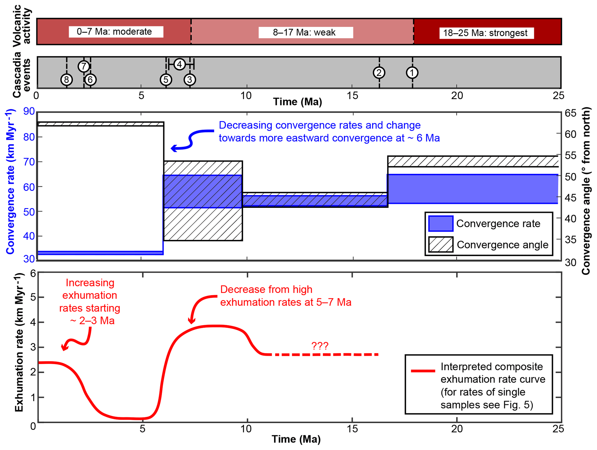
Figure 8Summary of volcanic activity, tectonic and climatic events, and convergence rate and angle at the Cascadia Subduction Zone in comparison with our interpreted exhumation rates for the past 25 Myr. Exhumation rates are limited to the time interval covered by our thermochronometric ages (0–11 Ma). The curve depicts the interpreted evolution of exhumation rates based on the modeling results shown in Fig. 5 (see text for details). Volcanic activity after du Bray and John (2011). Tectonic and climatic events are (1) the start of exhumation of the Olympic Mountains (Brandon et al., 1998), (2) the onset of uplift of the Oregon Coast Range (McNeill et al., 2000), (3) rotation in the stress field (Priest, 1990), (4) faster uplift in the Oregon Coast Range (McNeill et al., 2000), (5) Pacific-wide plate reorganization (Wilson, 2002), (6) the onset of North American glaciation (Haug et al., 2005), (7) the onset of glaciation within the Olympic Mountains (Easterbrook, 1986), and (8) a change in the deformational style of the offshore accretionary wedge (Flueh et al., 1998). Convergence rate and angle from Doubrovine and Tarduno (2008).
5.3 Temporal variations in exhumation
Our new thermo-kinematic modeling revealed temporal variations in exhumation rates in the Olympic Mountains (Fig. 5). The decrease in exhumation rates at 5–7 Ma can be readily explained by the reduction in plate convergence rate and the change in convergence direction (Fig. 8). A Pacific-wide reorganization of plate movement at 5.9 Ma has been suggested (Wilson, 2002), and rapid uplift of the Oregon Coast Range at 6–7.5 Ma with a subsequent cessation in uplift has also been attributed to variations in the plate subduction parameters (McNeill et al., 2000). Furthermore, the volcanic record of the Cascadia Subduction Zone shows temporal variations, and the strongest volcanic activity lasted from 25 until 18 Ma (du Bray and John, 2011). A period of volcanic quiescence, lasting from 17 until 8 Ma, was then followed by increased activity starting at ∼7 Ma. A change in the stress field of the Cascadia Subduction Zone occurred at 7 Ma, which likely also affected the composition of the magmatism (Priest, 1990). Therefore, we interpret our observed 5–7 Ma drop in exhumation rates in the Olympic Mountains as a response to changes in the plate tectonic conditions.
In contrast, the increase in exhumation rates at ∼2 Ma indicates a response to climatic rather than tectonic changes. As previously suggested by Michel et al. (2018), increased denudation due to the heavy glaciation of the mountain range led to an increase in exhumation rates by 50 %–150 % starting at 2–3 Ma. Our study corroborates these findings and shows that the observed young AHe ages require a recent increase in exhumation rates from slower rates (< 0.2 km Myr−1) lasting from ∼7 until ∼2 Ma. Glaciation of the North American continent commenced at 2.7 Ma (Haug et al., 2005) and the oldest glacial deposits within the Olympics could be as old as 2 Ma (Easterbrook, 1986), overlapping our modeled increase in rates at ∼2 Ma. Due to the strong spatial variation of the Pleistocene equilibrium line altitude within the Olympic Mountains (Porter, 1964), glacial erosion likely also varied spatially, which could explain the different magnitude of the increase in exhumation rates suggested for the different samples. Increased offshore sedimentation related to glacially eroded sediment affected the deformational style of the offshore wedge, leading to the formation of westward-dipping thrust faults, which changed at ∼1.5 Ma (Adam et al., 2004; Flueh et al., 1998; Gutscher et al., 2001).
Taken together, these observations indicate that temporal variations in exhumation rates within the Olympic Mountains are subject to changes in both the tectonic and climatic conditions (as summarized in Fig. 8). The implication of these variations should be considered for flux steady-state assessment.
5.4 Flux steady state in the Olympic Mountains
5.4.1 A qualitative perspective
Several variables that affect both the accretionary influx and the denudational outflux show temporal variations. Exhumation rates decrease at 5–7 Ma and increase at ∼2 Ma (Fig. 8), and since exhumation is primarily controlled by denudation, we equate these variations in exhumation with variations in the denudational outflux. According to the model of Doubrovine and Tarduno (2008), the plate subduction velocity decreased at ∼6 Ma (see Fig. 6b) after an earlier major decrease at ∼25 Ma, causing a decrease in the accretionary influx. Conversely, the accretionary influx increased significantly during the Quaternary due to high offshore sedimentation rates and increased sediment thicknesses as a result of effective glacial erosion on the North American continent (i.e., 50 %–70 % of the present-day sediment thickness on the subducting Juan de Fuca Plate consists of Quaternary-aged sediments; Table 1 and Fig. 3).
It follows that, qualitatively, both influx and outflux vary through time and are heavily influenced by the Plio–Pleistocene glaciation, which increased denudation rates and offshore sedimentation rates. However, we cannot quantitatively constrain whether variations in the influx and outflux on these short timescales (2–3 Myr) balance each other (and the system would still be in a flux steady state). Interestingly, measured denudation rates based on cosmogenic nuclide dating (temporally integrating over the Holocene) suggest that modern denudation rates have not been significantly influenced by Plio–Pleistocene glaciation, but are mostly driven by tectonic rock uplift (Adams and Ehlers, 2018). The Holocene accretionary influx, however, is still affected by the increased sediment thickness since the onset of glaciation. Hence, the current accretionary influx seems to exceed the denudational outflux in the Olympic Mountains.
5.4.2 A quantitative perspective
Here, we discuss the quantitative assessment of influx and outflux for the last 14 Myr (Table 5), the time since the Olympic Mountains are presumed to be in flux steady state (Batt et al., 2001; Brandon et al., 1998). In our geometry (Fig. 6a and d), we calculate the accretionary influx over a distance along the deformation front and the spatial exhumation rate pattern is integrated to infer the denudational outflux (Fig. 6d). Assuming an increase in sediment thickness at 2 Ma yields an accretionary volume (∼76 000 km3) similar to the denudational outflux (75 000–82 000 km3). Assuming a maximum sediment thickness of 2.5 km for the 14 Myr period yields an accretionary volume of ∼130 000 km3, which cannot be reconciled with our denudational outflux (Table 5). These results indicate that if temporal variations in the sediment thickness and denudation are considered, a reasonable balance between influx and outflux is attained. The previous flux steady-state analysis (Batt et al., 2001) was performed in two dimensions and used a constant sediment thickness of 2.0 km. We also performed an influx and outflux calculation using a two-dimensional geometry to tie in with previous work (see the Appendix). However, the results from the two-dimensional analysis suggest that for an area with spatially variable exhumation rates like the Olympic Mountains a three-dimensional geometry yields a more accurate prediction of influx and outflux.
Sediment volumes integrated along the cross sections (Fig. 7) also provide an interesting perspective on the accretionary influx in the Olympic Mountains. These volumes are not directly comparable with the influx–outflux volumes discussed above (calculated from 14–0 Ma) because the sediment contained within the cross sections (Fig. 7) records accretion since the ∼40 Ma onset of subduction (Brandon et al., 1998; du Bray and John, 2011). Furthermore, these estimates are minimum volumes because the amount of material that has been eroded during the 40 Myr period is not considered. Nevertheless, the amount of sediment currently residing in the accretionary wedge is variable along the strike of the subduction zone (1000–5400 km3) and is highest below the central part of the Olympic Mountains (Fig. 7). This requires that the parameters affecting the accretionary influx (like plate subduction velocity or sediment thickness) are highly variable over short distances (Profile 1 and Profile 2 are only 50 km apart; Fig. 7). Another explanation might be that considering accretion only perpendicular to the deformation is an oversimplification and another velocity component also contributes to material transport (see Sect. 5.5). This is in accordance with the conclusion drawn above that considering flux steady state in a two-dimensional scenario (as is done with the cross sections) leads to ambiguous results.
In summary, the assessment of flux steady state in the Olympic Mountains is nontrivial and several scenarios are possible. From a qualitative viewpoint, flux steady state is probably not achieved on short timescales (a few Myr) because the thickness of incoming sediment, plate subduction velocity, and exhumation rates show strong temporal variations on timescales of 2–3 Myr. From a quantitative viewpoint, influx and outflux volumes equate to each other over longer timescales (i.e., 14 Myr) if influx and outflux are considered in three dimensions.
5.5 Restrictions and limitations of our approaches
In the sections above, we discussed exhumation in the Olympic Mountains and the results from our flux calculations. In the following section, we want to elaborate on possible restrictions or limitations in our approaches.
With our 1-D modeling, we revealed strong temporal variations in exhumation rates (Fig. 5) related to variations in both tectonic and climatic conditions (Fig. 8). However, two of our modeled samples (OP1513 and OP1517) do not display the decrease in exhumation rates at ∼5–7 Ma. These are from the Elwha Valley (Fig. 4), in contrast to the five samples displaying the decrease, which are located in the western part of the mountain range. This suggests that the response of the orogenic wedge to a variation in the tectonic conditions affects only parts of the wedge and might be controlled by discrete structures. Further sampling and thermochronometric dating would be required to localize possible faults. Furthermore, this places a limitation on the application of a refined 3-D model because it requires constraining parameters such as fault location or displacement on these faults. Besides the importance of single structures, the general pattern of deformation in the Olympic Mountains should still be viewed as controlled by the geometry of the subducted plate (Adams and Ehlers, 2017, 2018; Brandon and Calderwood, 1990; Michel et al., 2018).
Regarding our flux analysis, we based our calculations on the volume of accreted sediment within a certain time (governed by the sediment thickness and the plate convergence rate) and the amount of denuded material (governed by the exhumation rates). As we mentioned in Sect. 3.3.1, a variable with great uncertainty is the sediment thickness over time, which has now been subducted below the Olympic Mountains. In the Supplement (Sect. S3.1) we outline our approach for assessing the pre-Quaternary sediment thickness, which is used in our calculations. Although the reported 1.5 km sediment thickness seems to be a plausible value, we note that this value is afflicted with uncertainties and might have been higher. Nonetheless, our proposed balance between influx and outflux is still tenable if the pre-Quaternary sediment thickness deviated from the assumed 1.5 km. In other words, we suggested an influx volume of 75–78×103 km3 and calculated outflux volumes between 75×103 and 82×103 km3 (Table 5), so even an additional influx volume due to a thicker, unnoticed sediment thickness could be balanced with our calculated outflux volumes. Another simplification in our calculation is the assumption of a spatially uniform sediment thickness over the considered length. Figure 3 shows that the sediment thickness along the deformation front is variable and is highest in the Nitinat and Astoria fans. However, an attempt to reconstruct along-strike variations in sediment thickness over time is challenging and would introduce further uncertainties, and thus we assume an average, constant thickness.
During our influx calculations, we did not distinguish between different modes of accretion, such as frontal accretion or underplating. Batt et al. (2001) concluded that most accretion occurs at the front of the wedge. However, a recent seismic study showed that sedimentary underplating is taking place below the Olympic Mountains (Calvert et al., 2011). For our approach, the mechanism of accretion does not matter because we are only interested in whether mass is balanced over the entire wedge and not at a specific point. As indicated, this is a limitation of our approach and might lead to an overestimation of the actual influx volume because we do not account for the amount of sediment transported towards the mantle.
Flux steady state implies that the outflux from and influx into a mountain range balance each other. An inherent assumption is often that the material removed from a mountain range (the outflux) again enters the mountain range via the influx, which consists of the denuded material from the same source. So in the case of an accretionary wedge, this implies that sediment is recycled and the system behaves as a closed system. As we described in Sect. 2.3 of the paper, the sediment currently entering the accretionary wedge of the Cascadia Subduction Zone is a mixture of sediment from different source regions (e.g., Olympic Mountains, Vancouver Island, Canadian Cordillera, and in the case of the Astoria fan, the interior USA; Fig. 3). With the increased detrital input from the Cordilleran Ice Sheet from outside the Olympic Mountains, this effect became particularly pronounced since the onset of Plio–Pleistocene glaciation. Hence, our influx–outflux calculations for the Olympic Mountains do not represent a closed system, and the influx into the Olympic Mountains is solely controlled by the outflux out of the system. However, our calculations indicate that on long timescales (i.e., over 14 Myr) flux steady state is attained, which might seem surprising given that the sediment thickness is governed by contributions from different source regions. We suspect that processes during sediment deposition, like redistribution by turbidity currents and redeposition in more proximal parts of the Juan de Fuca Plate, play an important role in the final sediment budget. As a consequence, the amount of sediment denuded from the Olympic Peninsula in a given time period (the outflux) is dispersed as it enters the ocean so that for the same time period only a fraction of the sediment thickness (governing the influx) is composed of material originating from the Olympic Peninsula.
Variations in the geometry or extent of the accretionary wedge were also not included in our flux analysis. Since the onset of subduction at the Cascadia Subduction Zone with the present geometry at ∼40 Ma, the wedge must have grown over time in order to attain its present shape. As soon as a balance between accretion and erosion is established, the shape of an orogenic wedge remains constant, controlled by its critical taper (e.g., Davis et al., 1983). However, Adam et al. (2004) showed that the Cascadia accretionary wedge responded to increased offshore sedimentation during the Quaternary through the development of westward-dipping thrust faults, shifting the deformation front further seawards, thereby increasing the extent and volume of the wedge. An important parameter contributing to the shape of the accretionary wedge is the angle of subduction, which is flatter below the Olympic Mountains (compared to areas north or south) due to the bend in the subducted slab (Fig. 1a). A reason hypothesized for bending the subducting slab is extension in the Basin and Range Province starting in the middle Miocene (Brandon and Calderwood, 1990). All these points indicate that parameters controlling the size and volume of the accretionary wedge are both spatially and temporally variable. However, we cannot account for all of these circumstances in our flux calculations because they are difficult to quantitatively constrain from available observations. Furthermore, because we based our flux calculations only on volumes of accreted or eroded material over the 14 Myr period, a comparison between these two volumes should not depend on a change in the shape or extent of the accretionary wedge.
As we pointed out in Sect. 5.4.2, flux steady state is obtained by using a three-dimensional geometry. However, we only considered the deformation front perpendicular velocity component for our influx calculations. The different sediment volumes contained in the reported cross sections (Fig. 7) could indicate that on long timescales additional velocity components must be considered. We can only speculate that margin-parallel transport, which is a contentious topic at the Cascadia Subduction Zone (e.g., Batt et al., 2001; McCrory, 1996; Wang, 1996), also contributes to the accretionary influx. Present-day GPS velocities corroborate this hypothesis, indicating northward movement of coastal areas south of the Olympic Mountains (e.g., McCaffrey et al., 2013; Wells and McCaffrey, 2013).
To summarize, several parameters, like the location of faults within the orogenic wedge, the sediment source region, the temporal evolution of the wedge geometry, and margin-parallel transport, are difficult to constrain from current observations. Although we emphasized that not all of these parameters affect our flux analysis, further knowledge of these will refine the current understanding of steady state in the Olympic Mountains.
Our new dataset of multi-dated thermochronometer bedrock samples together with thermo-kinematic modeling suggests that several mechanisms contribute to the evolution of the Olympic Mountains. Modeling of the observed AHe, AFT, ZHe, and ZFT ages shows that variations in both tectonic and climatic conditions result in temporal variations in exhumation rates. We revealed a hitherto unnoticed response of exhumation to the tectonic signal (a reduction in plate convergence rate causing a drop in exhumation rates), which can also be observed in other parts of the Cascadia Subduction Zone. Plio–Pleistocene glaciation of the Olympic Mountains led to increased denudation, resulting in increased exhumation rates.
Our approach of assessing flux steady state in the Olympic Mountains by estimating the material influx and outflux independently from each other is promising, but yields ambiguous results. The observed temporal variations in exhumation rate require a variation in the denudational outflux. Likewise, the accretionary influx is also temporally variable because the plate subduction velocity and incoming sediment thickness are variable through time. Qualitatively, this suggests that flux steady state is perturbed on short timescales by variations in the tectonic or climatic conditions. Our quantitative calculations of the influx and outflux show that flux steady state may be achievable over long timescales (i.e., 14 Myr). Contrary to a previous flux steady-state analysis in the Olympic Mountains, our calculated influx and outflux volumes only balance each other if a three-dimensional geometry is considered.
This study demonstrates the timescale (105–106 vs. 107 Myr) and spatial dependence of a steady-state assessment in an orogenic wedge. Furthermore, the tremendous effect of the Plio–Pleistocene glaciation is demonstrated, which is capable of significantly perturbing the development of an orogenic wedge, whereby both the influx and outflux are affected. Because we obtain flux steady state for a three-dimensional geometry (but only consider velocities parallel to the subduction direction), more work is needed to constrain the role of material transport parallel to the deformation front. Such studies will lead to a better understanding of the development of orogenic wedges situated in a complex tectonic setting like the Olympic Mountains.
All thermochronometry data used in this article are freely available and are either presented in the main paper or can be found in the Supplement. The exhumation histories derived from the modeling are displayed in Fig. 5, and the underlying data and scripts used to produce the figure are available from the authors.
In Sect. 3.3 we performed our flux analysis in three dimensions due to the spatially variable exhumation rates (Fig. 6d). In the following, we also calculate the influx and outflux using a two-dimensional geometry so that our calculations can be compared to those from Batt et al. (2001). Here, the accretionary influx occurs at a single location at the deformation front, and the sediment volume (Vsed2-D) is obtained by using a slightly modified version of Eq. (2):
Variables are porosity (η), incoming sediment thickness (d), time (t), and the deformation front perpendicular convergence rate (uper). The further procedure is identical to the procedure outlined in Sect. 3.3.1. Although the volumes obtained with this equation have a unit of km2, no great uncertainty is introduced if the analysis is expanded over a width of 1 km, which then yields values of km3 and “true” volumes. Calculated volumes are 520–540 km3 (for a 1.5 km thick sediment stack), 980–1020 km3 (for a 2.5 km thick sediment stack), and 580–600 km3 (for the increase in sediment thickness from 1.5 to 2.5 km at 2 Ma).
The outflux calculations are not based on the integration of the entire exhumation pattern in Fig. 6d, but rates are only integrated along the white line in Fig. 6. These integrals yield values of 68 km2 Myr−1 (constant rate), 103 km2 Myr−1 (50 % increase in rate), and 171 km2 Myr−1 (150 % increase in rate). After also integrating temporally (and assuming a width of 1 km in order to get units of km3; see above), the respective volumes of two-dimensional outflux are 900, 1000, and 1090 km3.
A comparison of two-dimensional influx and outflux shows that the accretionary influx (∼1000 km3) only balances the denudational outflux (1060–1160 km3) if an incoming sediment thickness of 2.5 km is assumed for the 14 Myr period. Hence, flux steady state can only be obtained using a two-dimensional geometry if an unrealistically high sediment thickness is assumed. Contrary to that, the three-dimensional geometry yields flux steady state using a more reasonable sediment thickness (an increase in sediment thickness from 1.5 to 2.5 km at 2 Ma). This indicates that assuming a two-dimensional geometry during the flux steady-state analysis is an oversimplification.
The supplement related to this article is available online at: https://doi.org/10.5194/esurf-7-275-2019-supplement.
LM, BA, and TE performed the fieldwork. Thermochronometric dating was done by CG, LM, and SF. LM performed the flux calculations with contributions from CG. The thermo-kinematic modeling was done by LM with help from BA and CG. LM drafted the initial versions of the paper and figures, and all authors commented on and contributed to the final version of the article.
The authors declare that they have no conflict of interest.
This work was funded by a European Research Council (ERC) Consolidator Grant
(615703) to Todd Ehlers. During fieldwork, we had invaluable help and
assistance from Holger Sprengel, William Baccus, Jerry Freilich, Roger Hofmann,
and the Olympic National Park rangers. We acknowledge Matthias Nettesheim for
sharing the code used for the evaluation of the tectonic plate reconstruction
model and the help of Willi Kappler during Pecube modeling. We thank
Associate Editor David Lundbek Egholm for editorial handling of the
paper. The comments by Phillipe Steer and one anonymous referee helped
to improve and clarify this paper.
Edited by: David Lundbek Egholm
Reviewed by: Philippe Steer and one anonymous referee
Adam, J., Klaeschen, D., Kukowski, N., and Flueh, E.: Upward delamination of Cascadia Basin sediment infill with landward frontal accretion thrusting caused by rapid glacial age material flux, Tectonics, 23, TC3009, https://doi.org/10.1029/2002TC001475, 2004.
Adams, B. A. and Ehlers, T. A.: Deciphering topographic signals of glaciation and rock uplift in an active orogen: a case study from the Olympic Mountains, USA: Signals of glaciation and rock uplift in the Olympic Mountains, Earth Surf. Proc. Land., 42, 1680–1692, https://doi.org/10.1002/esp.4120, 2017.
Adams, B. A. and Ehlers, T. A.: Tectonic controls of Holocene erosion in a glaciated orogen, Earth Surf. Dynam., 6, 595–610, https://doi.org/10.5194/esurf-6-595-2018, 2018.
Adams, B. A., Hodges, K. V., Whipple, K. X., Ehlers, T. A., van Soest, M. C., and Wartho, J.: Constraints on the tectonic and landscape evolution of the Bhutan Himalaya from thermochronometry: Late Cenozoic Evolution of Bhutan, Tectonics, 34, 1329–1347, https://doi.org/10.1002/2015TC003853, 2015.
Batt, G. E. and Brandon, M. T.: Lateral thinking: 2-D interpretation of thermochronology in convergent orogenic settings, Tectonophysics, 349, 185–201, https://doi.org/10.1016/S0040-1951(02)00053-7, 2002.
Batt, G. E., Brandon, M. T., Farley, K. A,. and Roden-Tice, M.: Tectonic synthesis of the Olympic Mountains segment of the Cascadia wedge, using two-dimensional thermal and kinematic modeling of thermochronological ages, J. Geophys. Res., 106, 26731–26746, https://doi.org/10.1029/2001JB000288, 2001.
Bendick, R. and Ehlers, T. A.: Extreme localized exhumation at syntaxes initiated by subduction geometry, Geophys. Res. Lett., 41, 2014GL061026, https://doi.org/10.1002/2014GL061026, 2014.
Bernard, T., Steer, P., Gallagher, K., Szulc, A., Whitham, A., and Johnson, C.: Evidence for Eocene–Oligocene glaciation in the landscape of the East Greenland margin, Geology, 44, 895–898, 2016
Berger, A. L., Gulick, S. P. S., Spotila, J. A., Upton, P., Jaeger, J. M., Chapman, J. B., Worthington, L. A., Pavlis, T. L., Ridgway, K. D., Willems, B. A., and McAleer, R. J.: Quaternary tectonic response to intensified glacial erosion in an orogenic wedge, Nat. Geosci., 1, 793–799, https://doi.org/10.1038/ngeo334, 2008.
Booth, D. B., Troost, K. G., Clague, J. J., and Waitt, R. B.: The Cordilleran Ice Sheet, in: Developments in Quaternary Sciences, 1, 17–43, Elsevier, 2003.
Booth-Rea, G., Klaeschen, D., Grevemeyer, I., and Reston, T.: Heterogeneous deformation in the Cascadia convergent margin and its relation to thermal gradient (Washington, NW USA), Tectonics, 27, TC4005, https://doi.org/10.1029/2007TC002209, 2008.
Brandon, M. T.: Decomposition of fission-track grain-age distributions, Am. J. Sci., 292, 535–564, 1992.
Brandon, M. T.: Probability density plot for fission-track grain-age sample, Radiat. Meas., 26, 663–676, 1996.
Brandon, M. T. and Calderwood, A. R.: High-pressure metamorphism and uplift of the Olympic subduction complex, Geology, 18, 1252, https://doi.org/10.1130/0091-7613(1990)018<1252:HPMAUO>2.3.CO;2, 1990.
Brandon, M. T. and Vance, J. A.: Tectonic evolution of the Cenozoic Olympic subduction complex, Washington State, as deduced from fission track ages for detrital zircons, Am. J. Sci., 292, 565–636, https://doi.org/10.2475/ajs.292.8.565, 1992.
Brandon, M. T., Roden-Tice, M. K., and Garver, J. I.: Late Cenozoic exhumation of the Cascadia accretionary wedge in the Olympic Mountains, northwest Washington State, Geol. Soc. Am. Bull., 110, 985–1009, https://doi.org/10.1130/0016-7606(1998)110<0985:LCEOTC>2.3.CO;2, 1998.
Braun, J.: Estimating exhumation rate and relief evolution by spectral analysis of age–elevation datasets, Terra Nova, 14, 210–214, 2002.
Braun, J.: Pecube: a new finite-element code to solve the 3-D heat transport equation including the effects of a time-varying, finite amplitude surface topography, Comput. Geosci., 29, 787–794, https://doi.org/10.1016/S0098-3004(03)00052-9, 2003.
Calvert, A. J., Preston, L. A., and Farahbod, A. M.: Sedimentary underplating at the Cascadia mantle-wedge corner revealed by seismic imaging, Nat. Geosci., 4, 545–548, https://doi.org/10.1038/ngeo1195, 2011.
Carpentier, M., Weis, D., and Chauvel, C.: Fractionation of Sr and Hf isotopes by mineral sorting in Cascadia Basin terrigenous sediments, Chem. Geol., 382, 67–82, https://doi.org/10.1016/j.chemgeo.2014.05.028, 2014.
Clague, J. J. and James, T. S.: History and isostatic effects of the last ice sheet in southern British Columbia, Quaternary Sci. Rev., 21, 71–87, 2002.
Clowes, R. M., Brandon, M. T., Green, A. G., Yorath, C. J., Brown, A. S., Kanasewich, E. R., and Spencer, C.: LITHOPROBE-southern Vancouver Island: Cenozoic subduction complex imaged by deep seismic reflections, Can. J. Earth Sci., 24, 31–51, 1987.
Davis, D., Suppe, J., and Dahlen, F. A.: Mechanics of fold-and-thrust belts and accretionary wedges, J. Geophys. Res., 88, 1153–1172, 1983.
Davis, E. E. and Hyndman, R. D.: Accretion and recent deformation of sediments along the northern Cascadia subduction zone, Geol. Soc. Am. Bull., 101, 1465–1480, 1989.
Doubrovine, P. V. and Tarduno, J. A.: A revised kinematic model for the relative motion between Pacific oceanic plates and North America since the Late Cretaceous, J. Geophys. Res., 113, TC4005, https://doi.org/10.1029/2008JB005585, 2008.
du Bray, E. A. and John, D. A.: Petrologic, tectonic, and metallogenic evolution of the Ancestral Cascades magmatic arc, Washington, Oregon, and northern California, Geosphere, 7, 1102–1133, 2011.
Easterbrook, D. J.: Stratigraphy and chronology of quaternary deposits of the Puget Lowland and Olympic Mountains of Washington and the Cascade Mountains of Washington and Oregon, Quaternary Sci. Rev., 5, 145–159, https://doi.org/10.1016/0277-3791(86)90180-0, 1986.
Eddy, M. P., Clark, K. P., and Polenz, M.: Age and volcanic stratigraphy of the Eocene Siletzia oceanic plateau in Washington and on Vancouver Island, Lithosphere, 9, 652–664, https://doi.org/10.1130/L650.1, 2017.
Ehlers, T. A.: Computational Tools for Low-Temperature Thermochronometer Interpretation, Rev. Mineral. Geochem., 58, 589–622, https://doi.org/10.2138/rmg.2005.58.22, 2005.
Ehlers, T. A., Farley, K. A., Rusmore, M. E., and Woodsworth, G. J.: Apatite (U-Th)/He signal of large-magnitude accelerated glacial erosion, southwest British Columbia, Geology, 34, 765–768, https://doi.org/10.1130/G22507.1, 2006.
Falkowski, S. and Enkelmann, E.: Upper-crustal cooling of the Wrangellia composite terrane in the northern St. Elias Mountains, western Canada, Lithosphere, 8, 359–378, https://doi.org/10.1130/L508.1, 2016.
Falkowski, S., Enkelmann, E., and Ehlers, T. A.: Constraining the area of rapid and deep-seated exhumation at the St. Elias syntaxis, Southeast Alaska, with detrital zircon fission-track analysis, Tectonics, 33, 597–616, https://doi.org/10.1002/2013TC003408, 2014.
Farley, K. A.: (U-Th)/He Dating: Techniques, Calibrations, and Applications, Rev. Mineral. Geochem., 47, 819–844, https://doi.org/10.2138/rmg.2002.47.18, 2002.
Fitzgerald, P. G., Stump, E., and Redfield, T. F.: Late Cenozoic uplift of Denali and its relation to relative plate motion and fault morphology, Science, 259, 497–497, 1993.
Flueh, E. R., Fisher, M. A., Bialas, J., Childs, J. R., Klaeschen, D., Kukowski, N., Parsons, T., Scholl, D. W., ten Brink, U., and Tréhu, A. M.: New seismic images of the Cascadia subduction zone from cruise SO108–ORWELL, Tectonophysics, 293, 69–84, 1998.
Galbraith, R. F.: Statistics for fission track analysis, CRC Press, 2005.
Gallagher, K., Brown, R., and Johnson, C.: Fission track analysis and its applications to geological problems, Annu. Rev. Earth Planet. Sci., 26, 519–572, https://doi.org/10.1146/annurev.earth.26.1.519, 1998.
Glotzbach, C., van der Beek, P., Carcaillet, J., and Delunel, R.: Deciphering the driving forces of erosion rates on millennial to million-year timescales in glacially impacted landscapes: An example from the Western Alps, J. Geophys. Res.-Earth, 118, 1491–1515, https://doi.org/10.1002/jgrf.20107, 2013.
Gulick, S. P. S., Jaeger, J. M., Mix, A. C., Asahi, H., Bahlburg, H., Belanger, C. L., Berbel, G. B. B., Childress, L., Cowan, E., Drab, L., Forwick, M., Fukumura, A., Ge, S., Gupta, S., Kioka, A., Konno, S., LeVay, L. J., März, C., Matsuzaki, K. M., McClymont, E. L., Moy, C., Müller, J., Nakamura, A., Ojima, T., Ribeiro, F. R., Ridgway, K. D., Romero, O. E., Slagle, A. L., Stoner, J. S., St-Onge, G., Suto, I., Walczak, M. D., Worthington, L. L., Bailey, I., Enkelmann, E., Reece, R., and Swartz, J. M.: Mid-Pleistocene climate transition drives net mass loss from rapidly uplifting St. Elias Mountains, Alaska, P. Natl. Acad. Sci. USA, 112, 15042–15047, https://doi.org/10.1073/pnas.1512549112, 2015.
Gutscher, M.-A., Klaeschen, D., Flueh, E., and Malavieille, J.: Non-Coulomb wedges, wrong-way thrusting, and natural hazards in Cascadia, Geology, 29, 379–382, 2001.
Han, S., Carbotte, S. M., Canales, J. P., Nedimović, M. R., Carton, H., Gibson, J. C., and Horning, G. W.: Seismic reflection imaging of the Juan de Fuca plate from ridge to trench: New constraints on the distribution of faulting and evolution of the crust prior to subduction, J. Geophys. Res.-Sol. Ea., 121, 1849–1872, https://doi.org/10.1002/2015JB012416, 2016.
Haug, G. H., Ganopolski, A., Sigman, D. M., Rosell-Mele, A., Swann, G. E. A., Tiedemann, R., Jaccard, S. L., Bollmann, J., Maslin, M. A., Leng, M. J. and Eglinton, G.: North Pacific seasonality and the glaciation of North America 2.7 million years ago, Nature, 433, 821–825, https://doi.org/10.1038/nature03332, 2005.
Hayes, G. P., Wald, D. J., and Johnson, R. L.: Slab1.0: A three-dimensional model of global subduction zone geometries, J. Geophys. Res.-Sol. Ea., 117, B01302, https://doi.org/10.1029/2011JB008524, 2012.
Herman, F. and Brandon, M.: Mid-latitude glacial erosion hotspot related to equatorial shifts in southern Westerlies, Geology, 43, 987–990, https://doi.org/10.1130/G37008.1, 2015.
Herman, F., Seward, D., Valla, P. G., Carter, A., Kohn, B., Willett, S. D., and Ehlers, T. A.: Worldwide acceleration of mountain erosion under a cooling climate, Nature, 504, 423–426, https://doi.org/10.1038/nature12877, 2013.
Hourigan, J. K., Reiners, P. W., and Brandon, M. T.: U-Th zonation-dependent alpha-ejection in (U-Th)/He chronometry, Geochim. Cosmochim. Ac., 69, 3349–3365, https://doi.org/10.1016/j.gca.2005.01.024, 2005.
Hurford, A. J.: Standardization of fission track dating calibration: Recommendation by the Fission Track Working Group of the I.U.G.S. Subcommission on Geochronology, Chem. Geol., 80, 171–178, 1990.
Hyndman, R. D. and Wang, K.: Thermal constraints on the zone of major thrust earthquake failure: The Cascadia Subduction Zone, J. Geophys. Res.-Sol. Ea., 98, 2039–2060, https://doi.org/10.1029/92JB02279, 1993.
Hyndman, R. D., Yorath, C. J., Clowes, R. M., and Davis, E. E.: The northern Cascadia subduction zone at Vancouver Island: Seismic structure and tectonic history, Can. J. Earth Sci., 27, 313–329, 1990.
Kiyokawa, S. and Yokoyama, K.: Provenance of turbidite sands from IODP EXP 1301 in the northwestern Cascadia Basin, western North America, Mar. Geol., 260, 19–29, https://doi.org/10.1016/j.margeo.2009.01.003, 2009.
Knudson, K. P. and Hendy, I. L.: Climatic influences on sediment deposition and turbidite frequency in the Nitinat Fan, British Columbia, Mar. Geol., 262, 29–38, https://doi.org/10.1016/j.margeo.2009.03.002, 2009.
Kulm, L. V. D., von Huene, R., Duncan, J. R., Ingle, J. C., Kling, S. A., Musich, L. F., Piper, D. J. W., Pratt, R. M., Schrader, H.-J., Weser, O. E., and Wise, S. W.: Site 174, edited by: Kulm, L. V. D., von Huene, R., Duncan, J. R., Ingle, J. C., Kling, S. A., Piper, D. J. W., Pratt, R. M., Schrader, H.-J., Wise, S. W., Musich, L. F., and Weser, O. E., Initial Reports of the Deep Sea Drilling Project, Publisher Texas A & M University, Ocean Drilling Program, College Station, TX, United States, 18, 97–167, https://doi.org/10.2973/dsdp.proc.18.1973, 1973.
Lease, R. O. and Ehlers, T. A.: Incision into the Eastern Andean Plateau During Pliocene Cooling, Science, 341, 774–776, https://doi.org/10.1126/science.1239132, 2013.
Lease, R. O., Haeussler, P. J., and O'Sullivan, P.: Changing exhumation patterns during Cenozoic growth and glaciation of the Alaska Range: Insights from detrital thermochronology and geochronology, Tectonics, 35, 934–955, https://doi.org/10.1002/2015TC004067, 2016.
Leeman, W. P., Lewis, J. F., Evarts, R. C., Conrey, R. M., and Streck, M. J.: Petrologic constraints on the thermal structure of the Cascades arc, J. Volcanol. Geoth. Res., 140, 67–105, https://doi.org/10.1016/j.jvolgeores.2004.07.016, 2005.
Lewis, T. J. and Bentkowski, W. H.: Potassium, Uranium and Thorium Concentrations of Crustal Rocks: a Data File, Open File Report 1744, Geological Survey of Canada, Sidney, 1988.
Lewis, T. J., Bentkowski, W. H., Davis, E. E., Hyndman, R. D., Souther, J. G., and Wright, J. A.: Subduction of the Juan de Fuca Plate: Thermal consequences, J. Geophys. Res.-Sol. Ea., 93, 15207–15225, https://doi.org/10.1029/JB093iB12p15207, 1988.
McCaffrey, R., King, R. W., Payne, S. J., and Lancaster, M.: Active tectonics of northwestern U.S. inferred from GPS-derived surface velocities, J. Geophys. Res.-Sol. Ea., 118, 709–723, https://doi.org/10.1029/2012JB009473, 2013.
McCrory, P. A.: Tectonic model explaining divergent contraction directions along the Cascadia subduction margin, Washington, Geology, 24, 929, https://doi.org/10.1130/0091-7613(1996)024<0929:TMEDCD>2.3.CO;2, 1996.
McCrory, P. A., Blair, J. L., Waldhauser, F., and Oppenheimer, D. H.: Juan de Fuca slab geometry and its relation to Wadati-Benioff zone seismicity, J. Geophys. Res.-Sol. Ea., 117, B09306, https://doi.org/10.1029/2012JB009407, 2012.
McNeill, L. C., Goldfinger, C., Kulm, L. D., and Yeats, R. S.: Tectonics of the Neogene Cascadia forearc basin: Investigations of a deformed late Miocene unconformity, Geol. Soc. Am. Bull., 112, 1209–1224, 2000.
Meesters, A. G. C. A. and Dunai, T. J.: A noniterative solution of the (U-Th)/He age equation, Geochem. Geophy. Geosy., 6, Q04002, https://doi.org/10.1029/2004GC000834, 2005.
Michel, L., Ehlers, T. A., Glotzbach, C., Adams, B. A., and Stübner, K.: Tectonic and glacial contributions to focused exhumation in the Olympic Mountains, Washington, USA, Geology, 46, 491–494, https://doi.org/10.1130/G39881.1, 2018.
Montgomery, D. R.: Valley formation by fluvial and glacial erosion, Geology, 30, 1047–1050, https://doi.org/10.1130/0091-7613(2002)030<1047:VFBFAG>2.0.CO;2, 2002.
Montgomery, D. R. and Greenberg, H. M.: Local relief and the height of Mount Olympus, Earth Surf. Proc. Land., 25, 385–396, 2000.
Mullen, E. K., Weis, D., Marsh, N. B., and Martindale, M.: Primitive arc magma diversity: New geochemical insights in the Cascade Arc, Chem. Geol., 448, 43–70, https://doi.org/10.1016/j.chemgeo.2016.11.006, 2017.
Mutz, S. G., Ehlers, T. A., Werner, M., Lohmann, G., Stepanek, C., and Li, J.: Estimates of late Cenozoic climate change relevant to Earth surface processes in tectonically active orogens, Earth Surf. Dynam., 6, 271–301, https://doi.org/10.5194/esurf-6-271-2018, 2018.
Pazzaglia, F. J. and Brandon, M. T.: A fluvial record of long-term steady-state uplift and erosion across the Cascadia forearc high, western Washington State, Am. J. Sci., 301, 385–431, 2001.
Phillips, B. A., Kerr, A. C., Mullen, E. K., and Weis, D.: Oceanic mafic magmatism in the Siletz terrane, NW North America: Fragments of an Eocene oceanic plateau?, Lithos, 274–275, 291–303, https://doi.org/10.1016/j.lithos.2017.01.005, 2017.
Porter, S. C.: Composite Pleistocene snow line of Olympic Mountains and Cascade Range, Washington, Geol. Soc. Am. Bull., 75, 477–482, 1964.
Priest, G. R.: Volcanic and tectonic evolution of the Cascade Volcanic Arc, central Oregon, J. Geophys. Res.-Sol. Ea., 95, 19583–19599, https://doi.org/10.1029/JB095iB12p19583, 1990.
Prytulak, J., Vervoort, J. D., Plank, T., and Yu, C.: Astoria Fan sediments, DSDP site 174, Cascadia Basin: Hf–Nd–Pb constraints on provenance and outburst flooding, Chem. Geol., 233, 276–292, https://doi.org/10.1016/j.chemgeo.2006.03.009, 2006.
Reiners, P. W., Zhou, Z., Ehlers, T. A., Xu, C., Brandon, M. T., Donelick, R. A., and Nicolescu, S.: Post-orogenic evolution of the Dabie Shan, eastern China, from (U-Th)/He and fission-track thermochronology, Am. J. Sci., 303, 489–518, 2003.
Reiners, P. W., Spell, T. L., Nicolescu, S., and Zanetti, K. A.: Zircon (U-Th)/He thermochronometry: He diffusion and comparisons with 40Ar/39Ar dating, Geochim. Cosmochim. Ac., 68, 1857–1887, https://doi.org/10.1016/j.gca.2003.10.021, 2004.
Stewart, R. J. and Brandon, M. T.: Detrital-zircon fission-track ages for the “Hoh Formation”: implications for late Cenozoic evolution of the Cascadia subduction wedge, Geol. Soc. Am. Bull., 116, 60–75, 2004.
Stolar, D., Roe, G., and Willett, S.: Controls on the patterns of topography and erosion rate in a critical orogen, J. Geophys. Res., 112, F04002, https://doi.org/10.1029/2006JF000713, 2007.
Stübner, K., Drost, K., Schoenberg, R., Böhme, M., Starke, J., and Ehlers, T. A.: Asynchronous timing of extension and basin formation in the South Rhodope core complex, SW Bulgaria, and northern Greece, Tectonics, 35, 136–159, https://doi.org/10.1002/2015TC004044, 2016.
Su, X., Baumann, K. H., and Thiede, J.: Calcareous nannofossils from Leg 168: biochronology and diagenesis, in Proceedings of the Ocean Drilling Program, Scientific Results, 168, 39–50, 2000.
Tabor, R. W. and Cady, W. M.: The structure of the Olympic Mountains, Washington: Analysis of a subduction zone, US Govt. Print. Off., 1978.
Thackray, G. D.: Extensive Early and Middle Wisconsin Glaciation on the Western Olympic Peninsula, Washington, and the Variability of Pacific Moisture Delivery to the Northwestern United States, Quaternary Res., 55, 257–270, https://doi.org/10.1006/qres.2001.2220, 2001.
Thiede, R. C. and Ehlers, T. A.: Large spatial and temporal variations in Himalayan denudation, Earth Planet. Sc. Lett., 371–372, 278–293, https://doi.org/10.1016/j.epsl.2013.03.004, 2013.
Thomson, S. N., Brandon, M. T., Tomkin, J. H., Reiners, P. W., Vásquez, C., and Wilson, N. J.: Glaciation as a destructive and constructive control on mountain building, Nature, 467, 313–317, https://doi.org/10.1038/nature09365, 2010.
Thomson, S. N., Reiners, P. W., Hemming, S. R., and Gehrels, G. E.: The contribution of glacial erosion to shaping the hidden landscape of East Antarctica, Nat. Geosci., 6, 203–207, https://doi.org/10.1038/ngeo1722, 2013.
Tomkin, J. H. and Roe, G. H.: Climate and tectonic controls on glaciated critical-taper orogens, Earth Planet. Sc. Lett., 262, 385–397, https://doi.org/10.1016/j.epsl.2007.07.040, 2007.
Valla, P. G., Shuster, D. L., and van der Beek, P. A.: Significant increase in relief of the European Alps during mid-Pleistocene glaciations, Nat. Geosci., 4, 688–692, https://doi.org/10.1038/ngeo1242, 2011.
Wang, K.: Simplified analysis of horizontal stresses in a buttressed forearc sliver at an oblique subduction zone, Geophys. Res. Lett., 23, 2021–2024, https://doi.org/10.1029/96GL02067, 1996.
Wells, R. E. and McCaffrey, R.: Steady rotation of the Cascade arc, Geology, 41, 1027–1030, https://doi.org/10.1130/G34514.1, 2013.
Wells, R. E., Bukry, D., Friedman, R., Pyle, D., Duncan, R., Haeussler, P., and Wooden, J.: Geologic history of Siletzia, a large igneous province in the Oregon and Washington Coast Range: Correlation to the geomagnetic polarity time scale and implications for a long-lived Yellowstone hotspot, Geosphere, 10, 692–719, 2014.
Westbrook, G. K., Carson, B., Musgrave, R. J., Ashi, J., Baranov, B., Brown, K. M., Camerlenghi, A., Caulet, J.-P., Chamov, N., Clenell, M. B., Cragg, B. A., Dietrich, P., Foucher, J.-P., Housen, B., Hovland, M., Jarrard R. D., Kastner, M., Kopf, A., MacKay, M. E., Moore, C., Moran, K., Parkes, R. J., Sample, J., Sato, T., Screaton, E. J., Tobin, H. J., Whiticar, M. J., Zellers, S. D.: Proceedings of the ODP, Initial Reports, 146 (Part 1), Texas A & M University, Ocean Drilling Program, College Station, TX , United States, 611 pp., https://doi.org/10.2973/odp.proc.ir.146-1.1994, 1994.
Whipple, K. X.: The influence of climate on the tectonic evolution of mountain belts, Nat. Geosci., 2, 97–104, https://doi.org/10.1038/ngeo413, 2009.
Whipple, K. X. and Meade, B.: Orogen response to changes in climatic and tectonic forcing, Earth Planet. Sc. Lett., 243, 218–228, https://doi.org/10.1016/j.epsl.2005.12.022, 2006.
Willett, S. D.: Orogeny and orography: The effects of erosion on the structure of mountain belts, J. Geophys. Res., 104, 28957–28981, https://doi.org/10.1029/1999JB900248, 1999.
Willett, S. D. and Brandon, M. T.: On steady states in mountain belts, Geology, 30, 175–178, https://doi.org/10.1130/0091-7613(2002)030<0175:OSSIMB>2.0.CO;2, 2002.
Willett, S. D., McCoy, S. W., Perron, J. T., Goren, L., and Chen, C.-Y.: Dynamic Reorganization of River Basins, Science, 343, 1248765–1248765, https://doi.org/10.1126/science.1248765, 2014.
Wilson, D. S.: Confidence intervals for motion and deformation of the Juan de Fuca Plate, J. Geophys. Res.-Sol. Ea., 98, 16053–16071, https://doi.org/10.1029/93JB01227, 1993.
Wilson, D. S.: The Juan de Fuca plate and slab: Isochron structure and Cenozoic plate motions, in: The Cascadia Subduction Zone and related subduction systems: seismic structure, intraslab earthquakes and processes, and earthquake hazards, US Geological Survey, Reston, VA, 2002.
Yanites, B. J. and Ehlers, T. A.: Global climate and tectonic controls on the denudation of glaciated mountains, Earth Planet. Sc. Lett., 325–326, 63–75, https://doi.org/10.1016/j.epsl.2012.01.030, 2012.
Yanites, B. J., Ehlers, T. A., Becker, J. K., Schnellmann, M., and Heuberger, S.: High magnitude and rapid incision from river capture: Rhine River, Switzerland, J. Geophys. Res.-Earth, 118, 1060–1084, https://doi.org/10.1002/jgrf.20056, 2013.
Yuan, T., Spence, G. D., and Hyndman, R. D.: Seismic velocities and inferred porosities in the accretionary wedge sediments at the Cascadia margin, J. Geophys. Res.-Sol. Ea., 99, 4413–4427, https://doi.org/10.1029/93JB03203, 1994.