the Creative Commons Attribution 4.0 License.
the Creative Commons Attribution 4.0 License.
 | 15 May 2019
Relationships between regional coastal land cover distributions and elevation reveal data uncertainty in a sea-level rise impacts model
Nathaniel G. Plant
E. Robert Thieler
Understanding land loss or resilience in response to sea-level rise (SLR) requires spatially extensive and continuous datasets to capture landscape variability. We investigate the sensitivity and skill of a model that predicts dynamic response likelihood to SLR across the northeastern US by exploring several data inputs and outcomes. Using elevation and land cover datasets, we determine where data error is likely, quantify its effect on predictions, and evaluate its influence on prediction confidence. Results show data error is concentrated in low-lying areas with little impact on prediction skill, as the inherent correlation between the datasets can be exploited to reduce data uncertainty using Bayesian inference. This suggests the approach may be extended to regions with limited data availability and/or poor quality. Furthermore, we verify that model sensitivity in these first-order landscape change assessments is well-matched to larger coastal process uncertainties, for which process-based models are important complements to further reduce uncertainty.
- Article
(1252 KB) - Full-text XML
-
Supplement
(563 KB) - BibTeX
- EndNote


Estimates of global sea-level rise (SLR) predict increases between 0.3 and 1.2 m by 2100 (Church et al., 2013; Kopp et al., 2014), while northeastern and mid-Atlantic US SLR projections are higher than the global average due to a variety of factors including subsidence, static equilibrium effects, and changing ocean dynamics (Goddard et al., 2015; Mitrovica et al., 2011; Kopp, et al., 2014; Sella et al., 2007; Slangen et al., 2014; Sweet et al., 2017a, b; Yin and Goddard, 2013; Yin et al., 2009; Zervas et al., 2013). SLR impacts such as high-tide flooding, barrier island narrowing, and salt marsh degradation have been increasingly observed along the US East Coast (e.g., Cahoon et al., 2009; Ezer and Atkinson, 2014; Kirwan and Megonigal, 2013; Sweet and Park, 2014). The northeastern US coast (from Maine southward through Virginia) is a diverse landscape, with major shipping ports (e.g., New York City, Boston, Norfolk), heavily populated cities (e.g., Washington, D.C., New York City, Boston), and extensive natural areas that provide a variety of habitat and ecosystem services. Understanding and assessing how coastal landscapes such as this respond to SLR is central to refining adaptive management strategies (Fishman et al., 2014) and identifying areas that provide buffering or mitigation to support long-term management targets (Pelletier et al., 2015).
Coastal environments are products of a complex interplay of exposure and processes, substrate and sediment supply, tidal ranges, and geomorphology (e.g., Davies, 1964; FitzGerald et al., 2008; Hayes, 1979). As illustrated by Carter (1988), a robust body of literature documents the ecologic transition of these environments from the shoreline over geomorphic features (e.g., dunes and bluffs) landward. In fact, a relatively steady SLR rate over the last few thousand years is central to our modern coastal configuration, including the development of barrier islands and wetlands (e.g., Redfield, 1972; Field and Duane, 1976; Shennan and Horton, 2002), as well as settlement patterns (McGranahan et al., 2007; Liu et al., 2015; Kane et al., 2017). Because coastal land elevation is primarily governed by the substrate and/or underlying geology of the landscape, as well as being a product of the physical and biogeochemical processes acting on it, it serves as a central parameter in defining the distribution and configuration of ecosystems and their ability to evolve in response to processes driving change (Gesch, 2009; Kempeneers et al., 2009).
Models are widely available (e.g., Marcy et al., 2011; Strauss et al., 2012) to estimate the potential for SLR-induced inundation across the landscape. These models use present-day elevation as a primary input, which makes them well-suited to identify impacts on developed areas, where hard structures, barriers to migration, and other stabilization measures constrain the landscape to its current elevation and use. However, these models cannot depict landscape variability in environments that respond dynamically to SLR through mechanisms such as vertical accretion due to washover or biomass accumulation. Lentz et al. (2016) addressed this limitation by developing a coastal response model (Fig. 2) for the northeastern US that predicts the likelihood of dynamic response to SLR, wherein dynamic is defined as the ability of an environment to either maintain its current state (e.g., a beach remains a beach) or transition to another non-submerged state (e.g., a forest becomes a marsh).
The confidence of our probabilistic dynamic response outcomes depends on the accuracy of model input parameters, which include continuous land cover and elevation data. Here, we use the nearly 38 000 km2 coverage of Lentz et al. (2016) to examine (1) the sensitivity of predictions to differences in the certainty of these input data and (2) model skill to determine where better data are necessary to improve prediction confidence and affect results. We explore the inherent correlation between elevation and coastal land cover distributions in our model by testing the ability of Bayesian inference to capture this relationship such that elevation may be used to predict land cover and vice versa. We hypothesize that the relationship between these data inputs over such an extensive and diverse expanse reduces uncertainty in each parameter in our framework and that potential data error is sufficiently minor that it does not obscure important process thresholds that would in turn affect predicted outcomes. In addition to better understanding model sensitivity to these parameters, our results also clarify how Bayesian inference may be used to supplement poorer data quality and/or uncertainty, particularly in low-lying coastal environments.
Table 1Summary table of accuracy rates for all confusion matrices of land cover and elevation comparisons. Accuracy rates are calculated by summing where predictions matched observations (the diagonal bolded terms in Tables S2–S4) and dividing by the total number of outcomes. Confusion matrices are available in the Supplement (Tables S2–S4).

2.1 Previous work
Lentz et al. (2015a) mapped coastal response predictions – the probability of dynamic response or DP – using a Bayesian network (BN) probabilistic modeling approach (Table 1). We define DP as the likelihood of land cover type to retain its existing state or transition to a new non-submerged state under the given SLR projection. By this definition, DP is a binary outcome in that if the coast does not respond dynamically to SLR, it will inundate, and therefore DP equals one minus the probability of inundation. A DP value of 0.5 indicated the highest uncertainty in that either dynamic response or inundation had an equally likely probability of occurrence (Lentz et al., 2016).
The study area was a 38 000 km2 region from Maine to Virginia, USA, bounded by the 10 m elevation contour inland to −10 m offshore. The BN (Fig. S1 in the Supplement) produced two probabilistic outcomes at a 30×30 m resolution for future SLR scenarios in the 2020s, 2030s, 2050s, and 2080s: (1) adjusted land elevation (AE) relative to the projected sea level and (2) dynamic response or DP. As described in Lentz et al. (2015a), the SLR scenarios were comprised of three components: ocean dynamics (generated from 24 Coupled Model Intercomparison Project Phase 5 (CMIP5) models; Taylor et al., 2012), ice melt (as estimated by Bamber and Aspinall, 2013, for the two Antarctic ice sheets and based on Marzion et al., 2012, and Radic et al., 2013, for glaciers and ice caps), and global land water storage (based on Church et al., 2013). Percentiles of these three components were estimated and then aggregated to provide an SLR scenario and corresponding uncertainty. The projected SLR scenario ranges for each decade used in our model are shown in Fig. S1 as follows: 2020s (0 to 0.25 m); 2030s (0.25 to 0.5 m); 2050s (0.5 to 0.75 m); and 2080s (0.75 to 2 m).
AE predictions were generated through implementation of a deterministic equation (see Fig. S1). First, SLR scenarios were combined with vertical land movement rates due to subsidence and other non-tectonic effects (using rates derived from a combination of GPS CORS stations in Sella et al., 2007, and long-term tide gauge data in Zervas et al., 2013) to make projections relative (local). Projected relative SLR values were then subtracted from elevation data binned in ranges (as shown in Fig. S1), which were comprised of a combination of high-resolution elevation data from the National Elevation Dataset (NED; Gesch, 2007) supplemented where necessary with coarser-resolution bathymetry from the National Oceanic and Atmospheric Administration National Geophysical Data Center's Coastal Relief Model (National Oceanic and Atmospheric Administration, 2014) to predict adjusted land elevation (AE) ranges relative to the projected sea level. Before model integration, high-resolution elevation data were converted to mean high water from the North American Vertical Datum 1988 using VDatum conversion grids (National Ocean Service, 2013).
Dynamic response probabilities (DP) were estimated by coupling the predicted AE ranges with expert knowledge on the response of generalized land cover types (six categories that respond distinctly to SLR ecologically or morphologically – subaqueous, marsh, beach, rocky, forest, and developed – as described in Lentz et al. (2015a) and shown in Table S1 in the Supplement). Although the resulting predictions provided a robust accounting of uncertainty from some of the data inputs and knowledge of physical landscape change processes, the relative influence of these uncertainties on the predictions has not been explored explicitly.
2.2 Sensitivity and skill assessment
We assessed the role of potential error in elevation (E) and land cover (LC) datasets on predicted outcomes. Beaches and estuarine wetlands exist near sea level; likewise, forests require elevations that provide adequate vadose zone thickness. While this correlation between E and LC allows one to be probabilistically predicted from the other, doing so also results in error correlation. Model elevation data came from the National Elevation Dataset (1∕9 or 1∕3 arcsec; U.S. Geological Survey, 2015) and Coastal Relief Model (as described in Lentz et al., 2015a). The expected errors in E from these data were included in previous predictions (Lentz et al., 2016), but their effect on predictions was not specifically addressed. Furthermore, the LC values (from McGarrigal et al., 2017) were not treated as uncertain, which was inconsistent with the treatment of all the other relationships in the Lentz et al. (2016) analysis. Better understanding of E and LC error helps to constrain it and identify where better data may improve predictions. Conversely, knowing where data have lower error helps to identify where process uncertainty is highest, which can help prioritize future research efforts.
We expanded our testing to determine (1) how our LC dataset compares with other LC data and previous error quantification results, (2) how E uncertainty is refined by LC information, and (3) where error in LC and E datasets is most likely to affect our predictions. As described in Lentz et al. (2016), inference training (Bayes' rule) was applied in the model to capture the correlation between E and LC in the form
where we evaluate the i outcome in the first term on the right as the probabilistic relationship conditioned on inputs from the j spatial location. Using this relationship, LC, entered with total certainty (such that P(LCj) is 1.0 if LCj corresponds to the land cover data at a particular location or P(LCj)=0.0 if it does not), updates the prior E, entered with known uncertainty, based on the values of the digital elevation model over the entire modeling domain. Similarly, E data are used to establish conditional probabilities of LC. By assessing potential E and LC error using a BN that implements Eq. (1) (Fig. S1), we can evaluate model skill in reducing error.
2.2.1 Land cover data comparison
As noted in Lentz et al. (2015a), the 2010 land cover data in the model (hereafter DSL, after McGarrigal et al., 2017) combine a variety of sources to capture detailed ecosystems information. To better evaluate land cover data error, we compared land cover data with the 2010 Coastal Change Analysis Program (CCAP) land cover dataset, which has a quantified error (NOAA, 2017, https://www.coast.noaa.gov/dataregistry/search/collection/info/ccapregional, last access: 19 October 2016) and was thus used as our “observed” data source. Although the DSL land cover data contain much more detailed ecosystem information than CCAP (19 classes in CCAP vs. 197 classes in DSL), our generalization of DSL data into six classes (Table S1) allowed us to similarly generalize CCAP data and compare the two datasets in terms of user error (accuracy, or how often the LC type in the DSL data would be the same in the CCAP or observed data) and producer error (reliability, or how often the LC type in the CCAP or observed data would be the same in the DSL data). When generalizing the two datasets for purposes of comparison, we further grouped together beach and rocky categories, as both exposed bedrock and beach–dune categories are included in the CCAP “bare land” category (Table S1). Data grids were compared using ArcGIS software's Combine tool (ESRI, 2016).
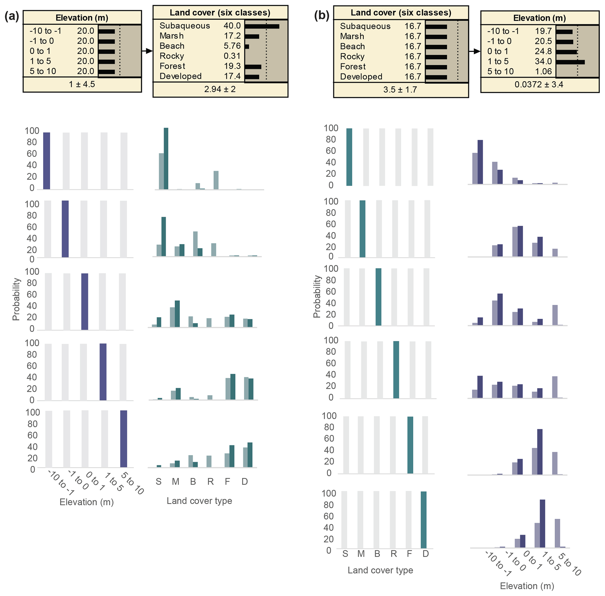
Figure 1Updated probability distributions after training between elevation and land cover datasets with nonuniform (dark) and uniform (light) priors (the latter to limit regional LC bias), (a) showing land cover distributions under selected elevation ranges and (b) elevation distributions under selected land cover types. Land cover categories (Table S1) are abbreviated as follows: S – subaqueous; M – marsh; B – beach; R – rocky; F – forest; and D – developed.
2.2.2 Model skill
Our training dataset included E and LC data at ∼42 000 000 grid cells throughout the northeast US. We tested our BN (developed with Netica software; Norsys Software Corp, 2013) and trained on these datasets, to predict E values from LC data and LC data from E values, by assessing posterior probability distributions in our BN and evaluating the error rate between predictions and observations. To perform this test, we built a separate two-variable BN to implement Eq. (1) consisting only of E and LC data (Fig. 1). The network was trained on the full elevation and DSL land cover dataset using Eq. (1), and an error rate was calculated based on the number of times the network predicted a value for a dataset that did not match the observed value at a given location. To test the extension of the inference relationship to situations in which E or LC data inputs may be unavailable or limited, the modified BN was used to predict an E value (or LC, as the BNs can be run as both forward and inverse models) as if it were unobserved given only the (uniformly distributed) LC data (or E value) as an input, and the corresponding posterior probabilities were observed.
2.2.3 Mismatch error
Some errors were expected from inconsistencies between the LC data and the E data, such as where subaqueous categories (Fig. 1) co-occurred with elevations above 0 m (referenced to mean high water, or MHW, in our model) and elevations below 0 m co-occurred with a land cover category other than subaqueous. These mismatches might be due to classification or elevation error, datum changes, or changes over time. To evaluate the impact of these mismatches, we focused on an area contained within the highest resolution and continuous elevation boundary contours (−1 to 10 m from the 1∕3 NED) using about half our points (∼22 000 000), as we anticipated that mismatch errors farther offshore than −1 m would be low (i.e., below 0 m and subaqueous). We classified mismatches by (1) E data resolution (1∕3 and, where available, 1∕9 arcsec data from the National Elevation Dataset) and (2) LC type to determine whether errors might be explained systematically due to inputs.
Once identified, we examined the effects of mismatches on the accuracy of predicted outcomes. First, our model was used to identify corresponding DP likelihood among LC types and the low-lying E ranges most commonly mistaken for one another (−1 to 0 and 0 to 1 m). Rather than evaluating a specific time step, we made input parameters defining relative SLR uniform (vertical land movement and projected sea level, as in Fig. S1) to assess overarching impacts on predictions. Mismatches were also compared geospatially with measured land cover shifts in the 2001 to 2010 CCAP change data (NOAA, 2013) to assess where E and LC data inputs, due to slightly differing dates in their data collection (Lentz et al., 2015a), may have captured dynamic state shifts due to process-based changes (e.g., movement of sand bodies around inlets or marsh erosion and/or inundation; Gomez et al., 2016).
3.1 Land cover error
Our LC error assessment found 15 % error between CCAP and DSL data; this value is the same as the published 15 % error for the CCAP dataset (Table 1 and McCombs et al., 2016). A confusion matrix (Table S2) reveals which LC classes were most commonly mistaken; the most frequent were bare land misclassified as subaqueous and marsh misclassified as non-marsh vegetation.
In addition to having the lowest number of pixels of all the land cover classes, user error and producer accuracy were lowest for the bare land category (49 % and 21 %, respectively); the lowest number of correctly classified pixels was in the bare land class when compared with the ground truth (CCAP) class. The bare land class also had the lowest number of pixels when compared with all other LC categories.
3.2 Model skill
The two-parameter BN showed that for this implementation, LC was nearly as useful for constraining E as the other way around (Fig. 1; Tables S3–S4). Figure 1a shows that when nonuniform E data were used to predict LC, subaqueous environments were the most probable prediction for elevations lower than 0 m (as illustrated by the top four plots on the left). This result reflects, in part, the dominance of subaqueous environments in our dataset and therefore the strong prior probability that any location below this elevation would be covered by water (Fig. S1). Additionally, we developed a modified BN with uniform prior distributions of LC (Fig. 1a) and E (Fig. 1b) to reevaluate the inference relationship as if all prior states of the nodes were equally probable, which limits prediction bias from the lower percentage representation of certain land cover categories in the region.
Generally (for both original and uniform prior BNs), elevation signatures specific to different land cover types were observed, with subaqueous, marsh, and beach environments appearing at low-lying elevations and developed and forested areas showing a predominance in higher-elevation settings (Fig. 1a). When relying on the original prior LC distribution, the network had a corresponding accuracy rate of 69 % (Table 1) and found beaches and rocky areas were not more probable than another land cover type. Here, beaches were most commonly confused with subaqueous and marsh land cover types and rocky areas with subaqueous (Table S3a). Uniformly distributed LC priors yielded slightly different predicted outcomes, wherein the network never found rocky and forested land cover types more probable than another land cover type, most commonly confusing them with subaqueous and developed land cover types, respectively (Table S3b). Overall, the accuracy rate in the inference relationship between E and LC was 56 % when uniform LC prior distributions were used (Table 1).
When land cover data were used to predict elevation (Fig. 1b), a consistent dependence of the E distribution on the LC data was seen, with E increasing as LC traversed submerged, marsh, beach, rocky, and forested environments. Overall, accuracy and reliability were lowest for the −1 to 0 and 0 to 1 m ranges with both original and uniform prior distributions of E (Tables S4a and b). The difference in prediction using the uniform prior BN was that the 5–10 m range category was predicted, whereas this elevation was not more probable than another when original priors were used. The accuracy rate in the inference relationship between LC and E was 66 % for the original prior distribution and 58 % for the uniform priors (Table 1).
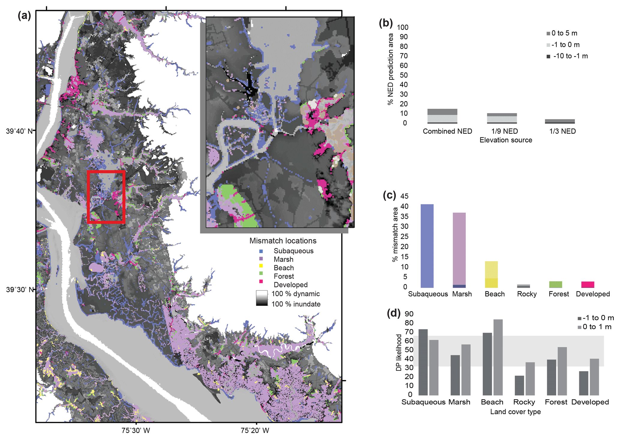
Figure 2Results of mismatch analysis (a) in a selected area with inset of enlarged view; (b) shown as a percentage of the prediction area within the 1∕3 National Elevation Dataset (NED) contour boundary and by elevation source type; (c) by land cover type as a percentage of the total mismatch area, where lighter hues show the percent of predictions in the −1 to 0 m range (with the exception of subaqueous, which shows a 0 to 1 m range), and darker hues show the percent of predictions in the −10 to 1 m range; and (d) the corresponding probability of dynamic response (DP) likelihood for each land cover type in the elevation ranges most commonly mistaken (light gray box shows the as likely as not likelihood range (0.33 > P > 0.66) following Mastrandrea et al., 2010).
3.3 Mismatch error
We define a mismatch as a location where the subaqueous LC type co-occurred with elevations above 0 m or where the remaining LC types co-occurred with elevations below 0 m. The mismatch assessment (Fig. 2a) showed that land–water mismatches affect 15 % of the reduced (> 19 000 km2) prediction area (Fig. 2b), and the most commonly occurring mismatches (Fig. 2c) were among dynamic environments (subaqueous, marshes, and beaches) at low elevations (−1 to 1 m). More than half of the mismatch data were comprised of LC categories other than subaqueous below 0 m. Of these, nearly all environments were found in the −1 to 0 bin, wherein marshes were the dominant environment type (35 % of mismatch), followed by beaches (8 % of mismatch). The remaining LC types (rocky, forest, developed) comprised < 6 % of the observed mismatch area combined. The cumulative probability of the subaqueous category falling into a positive E range (0 to 1 or 1 to 5 m) made up the remainder of the mismatch data (42 %), with nearly 78 % of these falling within the 0 to 1 m range.
Mismatches helped to highlight what may be systematic offsets with the E and LC data inputs. The most common mismatches were nearly evenly divided between 1∕3 and 1∕9 arcsec NED datasets; however, mismatch error was more dominantly comprised of elevation data below 0 m sourced to the 1∕9 arcsec NED, and error sourced to the 1∕3 arcsec dataset most commonly came from the subaqueous category falling into a positive E range. Mismatch error was also nearly 3 times as likely to occur in marshes or subaqueous categories as in any other LC category (Fig. 2b). In sum, mismatches were most concentrated in low-lying ranges for coastal areas (1) comprised of LC categories (beaches, marshes) most commonly misclassified in the LC comparison (Sect. 3.1) and (2) where land cover was most inaccurate and unreliable when used in predicting elevation (−1 to 1 m, Sect. 3.2). Using uncertainty terminology as in Mastrandrea et al. (2010), mismatched beaches had a likely DP (P > 0.66) in both −1 to 0 and 0 to 1 m bins (Fig. 2d), whereas the DP for the remaining mismatched land cover categories between −1 and 1 m were as likely as not (0.33 < P < 0.66; marshes, forests) to unlikely (P > 0.33; rocky, developed).
The high overall agreement between CCAP and DSL data when reclassified (Table S1) indicates DSL data have at most moderate error. Although the elevation data have a stated, calculated error that was integrated directly in our model, a similar error estimate was not available for the land cover (DSL) data (although our probabilistic framework allows this to be incorporated if available). Comparing the DSL land cover dataset to a dataset with a known error value (CCAP) revealed an identical error rate (15 %) to that determined for CCAP alone (McCombs et al., 2016). Although we cannot confirm that this error resides solely with the CCAP data, the updated and more detailed information in the DSL data, as well as the similarity in error rate with the published CCAP error, suggests that entering the DSL data as if they are known with certainty is an appropriate assumption for most of our LC categories.
The land cover comparison also showed that bare land and marsh categories are those most commonly classified as another category (subaqueous and non-marsh vegetation, respectively). The greatest error in the comparison – the bare land category – is in part explained by the substantial underrepresentation of beaches in both datasets when compared with other LC types. Due to this underrepresentation, beaches are never the most probable land cover type predicted from E when original prior distributions are applied (Table 3a). Our uniform prior test demonstrates that in spite of this regional bias, there is also ambiguity in the E–LC relationship with regards to beaches and marshes in our model; when either marshes are beaches are predicted from E with a uniform prior, they match the observed LC (user accuracy) 47 %–49 % of the time, respectively (Table S3b). However, beaches are more confidently predicted in the −1 to 0 m range than other land cover types (Fig. 1b), suggesting that a majority of beaches in our model training data are shallowly submerged. Incorporating first-return lidar instead of bare earth data in our model could further distinguish the six LC types from one another via vegetation differences (e.g., Lee and Shan, 2003; Im et al., 2008; Reif et al., 2011) and better distinguish intertidal areas, which may allow for the refinement of marsh, beach, and forest classifications (e.g., Kepeneers et al., 2009; Sturdivant et al., 2017).
Testing our two-node BN revealed that Bayesian inference can be used to fill data gaps or enhance data quality. Applying both nonuniform and uniform priors (the latter to remove the regional land cover biases specific to the northeastern US) showed that land-cover-specific elevation signatures are present. Notable distinctions were between elevation end-members (very high or very low relief; subaqueous, forests, developed) and midrange (moderate relief; marshes, beaches, rocky) areas. Assessing model skill in the E and LC relationship revealed an accuracy of 56 % (uniform priors) to 69 % (nonuniform priors), showing that including the regional LC bias helped to improve predictions (Table 1) and that the most commonly missed LC–E predictions occurred in elevations closest to mean sea level (−1 to 1 m).
In addition to missed predictions, our testing revealed that some E ranges and LC categories were never the most probable outcome. This was true for several land cover types (specifically, beaches and rocky under original E priors; rocky and forest under uniform priors; Tables S3) and one elevation range (5–10 m elevation under original LC priors; Table S4b). For the original priors, we attribute this to the underrepresentation of certain classes (regional bias) in our training data, wherein beaches, rocky, and 5–10 m elevation ranges were infrequent when compared to other classes or bins. In the case of uniform priors, our BN is detecting the slightly stronger relationship of some land cover types in certain elevation ranges (e.g., developed in the 1 to 5 m range), thereby making other E–LC relationships never more probable than these. Although bin reassignments that span smaller elevation ranges could help resolve more specific land cover signatures in our model, particularly for low-lying beaches and marshes, this would likely occur at the cost of increased prediction uncertainty as outcomes would span a larger number of bins.
Our mismatch analysis revealed that LC and E mismatches are uncommon and found at low elevations (−1 to 1 m) in dynamic environments (beaches, marshes, and subaqueous categories). Mismatches were most infrequent among typically higher-elevation environments (forests, developed, and rocky). We suggest that low-elevation mismatches resulted from physical changes, such as tidal inlets causing submerged sandbars to become subaerial beach or forests becoming marshes. However, comparison with CCAP changes from 2001 to 2010 revealed a very small (3 %) correspondence with identified areas of mismatch. Results instead may suggest that high-resolution (1∕9 NED) E data capture a systematic offset in part due to MHW submergence from datum conversion (Lentz et al., 2015a), particularly for marshes and beaches (Fig. 3b). In addition to elevation data that account for vegetation, as suggested earlier, seamless and continuous topographic and bathymetric data (Danielson et al., 2016) would constrain resolution error and better resolve distinctions between subaerial and subaqueous environments.
Ultimately, the contributions of data error are unlikely to change the DP uncertainty categories (Fig. 2d). In the case of LC error, the most commonly confused LC categories were subaqueous with beach categories and marshes with forests. In either case, when coupled with E data, beaches and subaqueous categories between −1 and 1 m generally have a likely DP and marshes and forests have an as likely as not DP (Fig. 2d), with the latter emphasizing the dominance of process uncertainty as accounted for in our original model via expert elicitation (as described in Lentz et al., 2015a) over data error in affecting DP outcomes. Furthermore, the response of developed and some beach areas to SLR is also particularly uncertain in our model due to unknowns regarding human behavior (Wong et al., 2014). Socioeconomic factors (McNamara et al., 2011; Hinkel et al., 2014) may determine where buildings and critical infrastructure are adapted to a dynamically changing landscape, coastal engineering projects are employed or upgraded (Gedan et al., 2011; Arkema et al., 2013), and alternatives such as inland migration (Hauer et al., 2016; Hauer, 2017) or managed retreat occur. Our probabilistic modeling framework allows us to update likelihood predictions as more information about the SLR response of the coastal landscape, and the people living on it, becomes available.
Our results show that (a) land cover error between two data sources is consistent with published error for one source (15 %), (b) inference training further reduces error, and (c) mismatch error is low with respect to the prediction area. To better resolve elevation and land cover distinctions in low-lying environments, elevation that accounts for vegetation distinctions and/or seamless datasets including both topography and bathymetry may be useful. However, the ability to capture the relationship between elevation and land cover via Bayesian inference in such a sizeable region demonstrates that it is possible to extend this application where data restrictions or gaps might otherwise limit expansion.
Furthermore, data input error has a minimal effect on our predicted outcomes, particularly when uncertainty terminology is applied (Fig. 2d). These outcomes therefore support first-order decision-making surrounding the inundation potential of specific environments, providing an essential risk assessment tool (NRC, 2009). We find that uncertainty in the response of different land cover types to varying SLR scenarios in our coastal response model is composed dominantly of uncertainty in physical and ecological processes, as opposed to data error, particularly for developed areas and low-elevation marshes (Lentz et al., 2016). To further refine assessments of future coastal response in areas of concern, data or deterministic models that account for site-specific SLR response rates and process knowledge will be well-paired with this approach.
Data for the coastal response outcomes referenced in this paper are published in the following repository: https://doi.org/10.5066/F73J3B0B (Lentz et al., 2015b).
The supplement related to this article is available online at: https://doi.org/10.5194/esurf-7-429-2019-supplement.
EEL and NGP designed the study, EEL conducted the analysis, and EEL, ERT, and NGP drafted the initial version of the paper. All authors discussed results and contributed to later versions of the paper.
The authors declare no that they have no conflicting interest.
This research was funded by the U.S. Geological Survey Coastal and Marine Geology Program. We thank P. Soupy Dalyander for early reviews and discussion of this paper. Any use of trade, firm, or product names is for descriptive purposes only and does not imply endorsement by the US Government.
This paper was edited by Paola Passalacqua and reviewed by two anonymous referees.
Arkema, K. K., Guannel, G., Verutes, G., Wood, S. A., Guerry, A., Ruckelshaus, M., Karejva, M., Lacayo, M., and Silver, J. M.: Coastal habitats shield people and property from sea-level rise and storms, Nat. Clim. Change, 3, 913–918, https://doi.org/10.1038/nclimate1944, 2013.
Bamber, J. L. and Aspinall, W. P.: An expert judgement assessment of future sea level rise from the ice sheets, Nat. Clim. Change, 3, 424–427, 2013.
Cahoon, D. R., Reed, D. J., Kolker, A. S., Brinson, M. M., Stevenson, J. C., Riggs, S., Christian, R., Reyes, E., Voss, C., and Kunz, D.: Coastal wetland sustainability, in: Coastal sensitivity to sea-level rise – A focus on the mid-Atlantic region, edited by: Titus, J. G., Anderson, K. E., Cahoon, D. R., Gesch, D. B., Gill, S. K., Gutierrez, B. T., Thieler, E. R., and Williams, S. J., Washington, D.C., U.S. Environmental Protection Agency, 57–72, 2009.
Carter, R.: Coastal environments: an introduction to the physical, ecological, and cultural systems of coastlines, Academic: San Diego, CA, 1988.
Church, J. A., Clark, P. U., Cazenave, A., Gregory, J. M., Jevrejeva, S., Levermann, A., Merrifield, M. A., Milne, G. A., Nerem, R. S., Nunn, P.D., Payne, A. J., Pfeffer, W. T., Stammer, D., and Unnikrishnan, A. S.: Sea level change, in: Climate Change 2013: The Physical Science Basis (Contribution of Working Group I to the Fifth Assessment Report of the Intergovernmental Panel on Climate Change), edited by: Stocker, T. F., Qin, D., Plattner, G.-K., Tignor, M., Allen, S. K., Boschung, J., Nauels, A., Xia, Y., Bex, V., and Midgley, P. M., Cambridge, United Kingdom and New York, NY, USA: Cambridge University Press, 2013.
Danielson, J. J., Poppenga, S. K., Brock, J. C., Evans, G. A., Tyler, D. J., Gesch, D. B., Thatcher, C. A., and Barras, J. A.: Topobathymetric elevation model development using a new methodology-Coastal National Elevation Database, J. Coast. Res., 76, 75–89, https://doi.org/10.2112/SI76-008, 2016.
Davies, J. L.: A morphogenic approach to world shorelines, Z. Geomorphol., 8, 27–42, 1964.
ESRI: ArcGIS Desktop: Release 10, Redlands, CA: Environmental Systems Research Institute, 2016.
Ezer, T. and Atkinson, L. P.: Accelerated flooding along the U.S. East Coast: On the impact of sea-level rise, tides, storms, the Gulf Stream, and the North Atlantic Oscillations, Earth's Future, 2, 362–382, 2014.
Fischman, R. L., Meretsky, V. J., Babko, A., Kennedy, M., Liu, L., Robinson, M., and Wambugu, S.: Planning for adaptation to climate change: Lessons from the US National Wildlife Refuge System, BioScience, 64, 993–1005, 2014.
FitzGerald, D. M., Fenster, M. S., Argow, B. A., and Buynevich, I. V.: Coastal impacts due to sea-level rise, Annu. Rev. Earth Planet. Sc., 36, 601–647, 2008.
Field, M. E. and Duane, D. B.: Post-Pleistocene history of the United States inner continental shelf: Significance to origin of barrier islands, Geol. Soc. Am. Bull., 87, 691–702, 1976.
Gedan, K. B., Kirwan, M. L., Wolanski, E., Barbier, E. B., and Silliman, B. R: The present and future role of coastal wetland vegetation in protecting shorelines: Answering recent challenges to the paradigm, Clim. Change, 106, 7–29, 2011.
Gesch, D. B.: The national elevation dataset, chap. 4 of Maune, edited by: Maune, D. F., Digital elevation model technologies and applications – The DEM users manual, 2d ed., 99–118, Bethesda, Md., American Society for Photogrammetry and Remote Sensing, 2007.
Gesch, D. B.: Analysis of lidar elevation data for improved identification and delineation of lands vulnerable to sea-level rise, J. Coast. Res., 53, 49–58, 2009.
Goddard, P. B., Yin, J., Griffies, S. M., and Zhang, S.: An extreme event of sea-level rise along the Northeast coast of North America in 2009–2010, Nat. Commun., 6, 6346, https://doi.org/10.1038/ncomms7346, 2015.
Gomez, C., White, J. C., and Wulder, M. A.: Optical remotely sensed time series data for land cover classification: A review, ISPRS J. Photogramm., 116, 55–72, 2016.
Hauer, M. E.: Migration induced by sea-level rise could reshape the US population landscape, Nat. Clim. Change, 7, 321–325, 2017.
Hauer, M. E., Evans, J. M., and Mishra, D. R.: Millions projected to be at risk from sea-level rise in the continental United States, Nat. Clim. Change, 6, 691–695, 2016.
Hayes, M. O.: Barrier island morphology as a function of tidal and wave regime, in: Barrier Islands from the Gulf of St. Lawrence to the Gulf of Mexico, edited by: Leatherman, S. P., 1–27, New York, NY, Academic, 1979.
Hinkel, J., Lincke, D., Vafeidis, A. T., Perrette, M., Nicholls, R. J., Tol, R. S. J., Marzeion, B., Fettweis, X., Ionescu, C., and Levermann, A.: Coastal flood damage and adaptation costs under 21st century sea-level rise, P. Natl. Acad. Sci. USA, 111, 3292–3297, 2014.
Im, J., Jensen, J. R., and Hodgson, M. E.: Object-based land cover classification using high-posting-density lidar data, GIScience and Remote Sensing, 45, 209–228, 2008.
Kane, H., Fletcher, C., Cochrane, E., Mitrovica, J., Habel, S., and Barbee, M.: Coastal plain stratigraphy records tectonic, environmental, and human habitability changes related to sea-level drawdown, Upolu, Samoa, Quaternary Res., 87, 246–257, 2017.
Kempeneers, P. Deronde, B., Provoost, S., and Houthuys, R.: Synergy of airborne digital camera and lidar data to map coastal dune vegetation, J. Coast. Res., 53, 73–82, 2009.
Kirwan, M. L. and Megonigal, J. P.: Tidal wetland stability in the face of human impacts and sea-level rise, Nature, 504, 53–60, 2013.
Kopp, R. E., Horton, R. M., Little, C. M., Mitrovica, J. X., Oppenheimer, M., Rasmussen, D. J., Strauss, B. H., and Tebaldi, C.: Probabilistic 21st and 22nd century sea-level projections at a global network of tide-gauge sites, Earth's Future, 2, 383–406, 2014.
Lee, D. S. and Shan, J.: Class-guided building extraction from Ikonos imagery, Photogramm. Eng. Rem. S., 2, 143–150, 2013.
Lentz, E. E., Stippa, S. R., Thieler, E. R., Plant, N. G., Gesch, D. B., and Horton, R. M.: Evaluating coastal landscape response to sea-level rise in the northeastern United States – Approach and methods, OFR 2014-1252, U.S. Geological Survey, 2015a.
Lentz, E. E., Stippa, S. R., Thieler, E. R., Plant, N. G., Gesch, D. B., and Horton, R. M.: Coastal landscape response to sea-level rise assessment for the northeastern United States (ver. 2.0., December 2015): U.S. Geological Survey data release, https://doi.org/10.5066/F73J3B0B, 2015b.
Lentz, E. E., Thieler, E. R., Plant, N. P., Stippa, S. R., Horton, R., and Gesch, D. B.: Evaluation of dynamic coastal response to sea-level rise modifies inundation likelihood, Nat. Clim. Change, 6, 696–700, 2016.
Liu, J., Wen, J., Huang, Y., Shi, M., Meng, Q., Ding, J., and Xu, H.: Human settlement and regional development in the context of climate change: A spatial analysis of low elevation coastal zones in China, Mitig. Adapt. Strat. Gl., 20, 527–546, 2015.
Marcy, D, Brooks, W., Draganov, K., Hadley, B., Haynes, C., Herold, N., McCombs, J., Pendleton, M., Ryan, S., Schmid, K., Sutherland, M., and Waters, K.: New mapping tool and techniques for visualizing sea-level rise and coastal flooding impacts, in: Solutions to Coastal Disasters 2011, edited by: Wallendorf, L., Jones, C., Ewing, L., and Battalio, B., American Society of Civil Engineers, Reston, VA, 474–490, 2011.
Marzeion, B., Jarosch, A. H., and Hofer, M.: Past and future sea-level change from the surface mass balance of glaciers, The Cryosphere, 6, 1295–1322, https://doi.org/10.5194/tc-6-1295-2012, 2012.
Mastrandrea, M. D., Field, C. B., Stocker, T. F., Edenhofer, O., Ebi, K. L., Frame, D. J., Held, H., Kriegler, E., Mach, K. J., Matschoss, P. R., Plattner, G.-K., Yohe, G. W., and Zwiers, F. W.: Guidance Note for Lead Authors of the IPCC Fifth Assessment Report on Consistent Treatment of Uncertainties, Intergovernmental Panel on Climate Change (IPCC), 2010.
McCombs, J. W., Herold, N. D., Burkhalter, S. G., and Robinson, C. J.: Accuracy assessment of NOAA Coastal Change Analysis Program 2006–2010 Land Cover and Land Cover Change Data, Photogramm. Eng. Rem. S., 82, 711–718, 2016.
McGarigal, K., Compton, B. W., Plunkett, E. B., Deluca, W. V., and Grand, J.: Designing sustainable landscapes: DSLland and Subsysland, Report to the North Atlantic Conservation Cooperative, US Fish and Wildlife Service, Northeast Region, available at: http://jamba.provost.ads.umass.edu/web/LCC/DSL_documentation_DSLland.pdf (last access: 28 November 2018), 2017.
McGranahan, G., Balik, D., and Anderson, B.: The rising tide: assessing the risks of climate change and human settlements in low elevation coastal zones, Environ. Urban., 19, 17–37, 2007.
McNamara, D. E., Murray, A. B., and Smith, M. D.: Coastal sustainability depends on how economic and coastline responses to climate change affect each other, Geophys. Res. Lett., 38, L07401, https://doi.org/10.1029/2011GL047207, 2011.
Mitrovica, J. X., Gomez, N., Morrow, E., Hay, C., Latychev, K., and Tamisiea, M. E.: On the robustness of predictions of sea level fingerprints, Geophys. J. Int., 187, 729–742, 2011.
National Oceanic and Atmospheric Administration National Geophysical Data Center: U.S. coastal relief model: National Oceanic and Atmospheric Administration National Geophysical Data Center Web page, available at: https://www.ngdc.noaa.gov/mgg/coastal/crm.html, last access: 9 June 2014.
National Oceanic and Atmospheric Administration, Office for Coastal Management: 2010 Coastal Change Analysis Program (C-CAP) Regional Land Cover, available at: https://www.coast.noaa.gov/ccapftp, last access: 5 June 2017.
National Ocean Service: VDatum manual for development and support of NOAA's vertical datum transformation tool, VDatum (ver. 1.01): National Oceanic and Atmospheric Administration and National Geodetic Survey, 119 pp., available at: http://vdatum.noaa.gov/docs/publication.html, last access: 19 December 2013.
National Research Council: Science and Decisions: Advancing Risk Assessment, The National Academies Press, Washington DC, USA, 422 pp., 2009.
NOAA's Coastal Change Analysis Program (C-CAP) 2001 to 2010 Regional Land Cover Change Data – Coastal United States: Department of Commerce (DOC), National Oceanic and Atmospheric Administration (NOAA), National Ocean Service (NOS), Office for Coastal Management (OCM), available at: https://coast.noaa.gov/dataregistry/search/dataset/info/ccapregional (last access: 5 June 2017), 2013.
Norsys Software Corp: Netica 5.12, Bayesian network development software, available at: https://www.norsys.com/ (last access: 12 March 2019), 2013.
Pelletier, J. D., Murray, A. B., Pierce, J. L., Bierman, P. R., Breshears, D. D., Crosby, B. T., Ellis, M., Foufoula-Georgiou, E., Himsath, A. M., Houser, C., Lancaster, N., Marani, M., Merritts, D. J., Moore, L. J., Pederson, J. L., Poulous, M. J., Rittenour, T. M., Rowland, J. C., Ruggiero, P., Ward, D. J., Wickert, A. D., and Yager, E. M.: Forecasting the response of Earth's surface to future climatic and land use changes: A review of methods and research needs, Earth's Future, 3, 220–251, 2015.
Radić, V., Bliss, A., Beedlow, C. D., Hock, R., Miles, E., and Cogley, J. G.: Regional and global projections of twenty-first century glacier mass changes in response to climate scenarios from global climate models, Clim. Dynam., 42, 37–58, 2013.
Redfield, A. C.: Development of a New England salt marsh, Ecol. Monogr., 42, 201–237, 1972.
Reif, M. K., Macon, C. L., and Wozencraft, J. M.: Post-Katrina land cover, elevation, and volume change assessment along the south shore of Lake Pontchartrain, Louisiana, USA, J. Coast. Res., 62, 30–39, 2011.
Sella, G. F., Stein, S., Dixon, T. H., Craymer, M., James, T. S., Mazzotti, S., and Dokka, R. K.: Observation of glacial isostatic adjustment in “stable” North America with GPS, Geophys. Res. Lett., 34, L02306, https://doi.org/10.1029/2006GL027081, 2007.
Shennan, I. and Horton, B.: Holocene land- and sea-level changes in Great Britain, J. Quaternary Sci., 17, 511–526, 2002.
Slangen, A. B. A., Church, J. A., Zhang, X., and Monselesan, D.: Detection and attribution of global mean thermosteric sea level change, Geophys. Res. Lett., 41, 5951–5959, 2014.
Strauss, B. H., Ziemlinski, R., Weiss, J. L., and Overpeck, J. T.: Tidally adjusted estimates of topographic vulnerability to sea level rise and flooding for the contiguous U.S., Environ. Res. Lett., 7, 014033, https://doi.org/10.1088/1748-9326/7/1/014033, 2012.
Sturdivant E., Lentz E. E., Thieler, E. R., Farris, A., Weber, K., Remsen, D., Miner, S., and Henderson R.: UAS-SfM for coastal research: Geomorphic feature extraction and land cover classification from high-resolution elevation and optical imagery, Remote Sens., 9, 1020, https://doi.org/10.3390/rs9101020, 2017.
Sweet, W. V. and Park, J.: From the extreme to the mean: Acceleration and tipping points of coastal inundation from sea level rise, Earth's Future, 2, 579–600, 2014.
Sweet, W. V., Kopp, R. E., Weaver, C. P., Obeysekera, J., Horton, R. M., Thieler, E. R., and Zervas, C.: Global and Regional Sea Level Rise Scenarios for the United States, NOAA Technical Report NOS CO-OPS 083, NOAA/NOS Center for Operational Oceanographic Products and Services, 75 pp., 2017a.
Sweet, W. V., Horton, R., Kopp, R. E., LeGrande, A. N., and Romanou, A.: Sea Level Rise, in: Climate Science Special Report: Fourth National Climate Assessment, edited by: Wuebbles, D. J., Fahey, D. W., Hibbard, K. A., Dokken, D. J., Stewart, B. C., and Maycock, T. K., Volume 1, 333–363, U.S. Global Change Research Program: Washington DC, 2017b.
Taylor, K. E., Stouffer, R. J., and Meehl, G. A.: An overview of CMIP5 and the experiment design, B. Am. Math. Soc., 93, 485–498, 2012.
U.S. Geological Survey: NED spatial metadata, available at: https://ned.usgs.gov/downloads.html, last access: 2 January 2015.
Wong, P. P., Losada, I. J., Gattuso, J.-P., Hinkel, J., Khattabi, A., McInnes, K. L., Saito, Y., and Sallenger, A.: Coastal systems and low-lying areas, in: Climate Change 2014: Impacts, Adaptation, and Vulnerability. Part A: Global and Sectoral Aspects, edited by: Field, C. B., Barros, V. R., Dokken, D. J., Mach, K. J., Mastrandrea, M. D., Bilir, T. E., Chatterjee, M., Ebi, K. L., Estrada, Y. O., Genova, R. C., Girma, B., Kissel, E. S., Levy, A. N., MacCracken, S., Mastrandrea, P. R., and White, L. L.: Contribution of Working Group II to the Fifth Assessment Report of the Intergovernmental Panel on Climate Change, Cambridge University Press: Cambridge, United Kingdom and New York, NY, USA, 361–409, 2014.
Yin, J. and Goddard, P. B.: Oceanic control of sea level rise patterns along the East Coast of the United States, Geophys. Res. Lett., 40, 5514–5520, 2013.
Yin, J., Schlesinger, M. E., and Stouffer, R. J.: Model projections of rapid sea-level rise on the northeast coast of the United States, Nat. Geosci., 2, 262–266, 2009.
Zervas, C., Gill, S., and Sweet, W.: Estimating Vertical Land Motion from Long-Term Tide Gauge Records, NOAA Technical Report NOS CO-OPS 065, 30 pp., 2013.