During the 2016–2017 winter season, we installed two seismic arrays above Davos, Switzerland (Fig. 1). The arrays were similar to the system described by van Herwijnen and Schweizer (2011a). The first array was deployed at the Dischma field site (yellow square in Fig. 1), 14 km from Davos at the end of a tributary valley (Heck et al., 2019). The field site is a flat meadow at an elevation of 2000 m a.s.l. surrounded by mountain peaks which rise up to 3000 m. The second array was deployed at the Wannengrat field site above Davos at 2400 m a.s.l. (red square in Fig. 1). This field site is surrounded by several avalanche starting zones (van Herwijnen and Schweizer, 2011a). Both arrays consisted of a 300 m long string with seven vertical component geophones with a natural frequency of 4.5 Hz. The sensors of the Dischma array were buried at a depth of about 50 cm, whereas the sensors at the Wannengrat field site were attached to rocks using an anchor. For each array, the sensors were circularly arranged (Fig. 1). The maximum distances between two sensors at the Dischma and Wannengrat field sites were 64 and 74 m, respectively, and the average distances were 36 and 45 m, respectively.

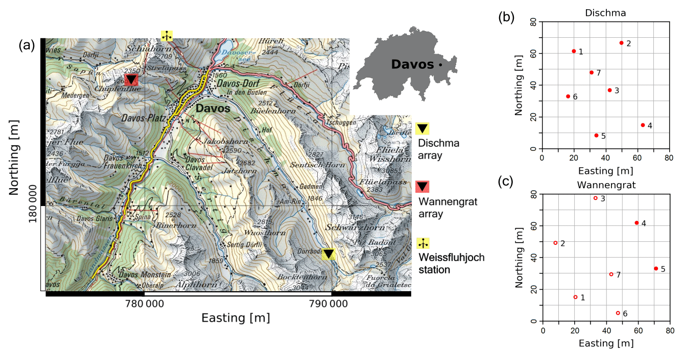
Figure 1(a) Map of the Davos area, Switzerland. The two seismic arrays are indicated by black triangles on different colored backgrounds: red represents the Wannengrat array, yellow represents the Dischma array. The wind wheel at the top of the panel indicates the location of the Weissfluhjoch weather station. (b) The deployment geometry of the Dischma array. (c) The deployment geometry of the Wannengrat array. The open red circles indicate the positions of malfunctioning sensors during winter 2017. Reproduced with permission from Swisstopo (JA100118).

Download

The instrumentation and data logging systems were identical for both arrays. Data were continuously recorded at a sampling rate of 500 Hz. Due to technical problems, only two sensors from the Wannengrat array recorded data throughout the entire winter (sensors 4 and 5 in Fig. 1b), and no data were collected between 12 and 20 January 2017. Both field sites were also equipped with several automatic cameras (eight at Dischma and six at Wannengrat) to monitor the surrounding slopes (Fig. 2). Images were recorded every 10 min throughout the winter. In addition, we also performed a field survey at the Dischma site on 15 March 2017 shortly after a period of high avalanche activity to identify avalanches and map their outlines (Fig. 3) (Heck et al., 2019).

Figure 2(a) Detailed map of the Dischma field site showing the position of the seismic array and the automatic cameras. (b) Same as (a), but for the Wannengrat field site. Reproduced with permission from Swisstopo (JA100118).

Download

Figure 3Picture of the Dischma field site facing south. The picture was taken on 15 March 2017 shortly after a period of high avalanche activity and several recent avalanches were observed (red areas). The triangle indicates the location of the seismic array, and the camera icon indicates the location of the automatic camera.

Download

The overall goal was to develop a processing workflow to automatically identify avalanches in seismic data from the Dischma field site by combining HMMs with seismic array processing techniques. The developed workflow consists of five steps which are described in more detail below (Fig. 4): (1) preprocessing, (2) feature calculation, (3) HMM construction, (4) classification and (5) post-processing.

Figure 4Flow chart of the classification process. Green lines show the construction of the event model, blue lines show the construction of the background model and orange lines show how the data to be classified are processed.

Download

3.3 HMM construction

The hidden Markov models that we used to automatically identify avalanches in the continuous seismic data consisted of a background model and an event model for each event class (Hammer et al., 2017; Heck et al., 2018). In our application we only used one event class, either avalanches at the Dischma field site or airplanes at the Wannengrat field site.

The background model can also be trained using features extracted from the preprocessed data. Previous work has shown that a background model which is regularly updated provides better classification results throughout a season (e.g., Heck et al., 2018). Hence, in our case, we used the preprocessed data from a 24 h window to train the background model and recalculated it every hour, i.e., we used a sliding window with a length of t_model=24 h and then shifted it forward by 1 h (background data in Fig. 4).

In contrast to the background model, the event model was only calculated once for the entire season (training event in Fig. 4). For the Dischma field site, our training event consisted of a signal generated by an avalanche that was released on 9 March 2017 at 06:47 LT (Fig. 5a), an unambiguous event that was analyzed in detail by Heck et al. (2019). For the Wannengrat field site, our training event consisted of a signal generated by an airplane on 31 January 2017 at 21:46 LT (Fig. 5b).

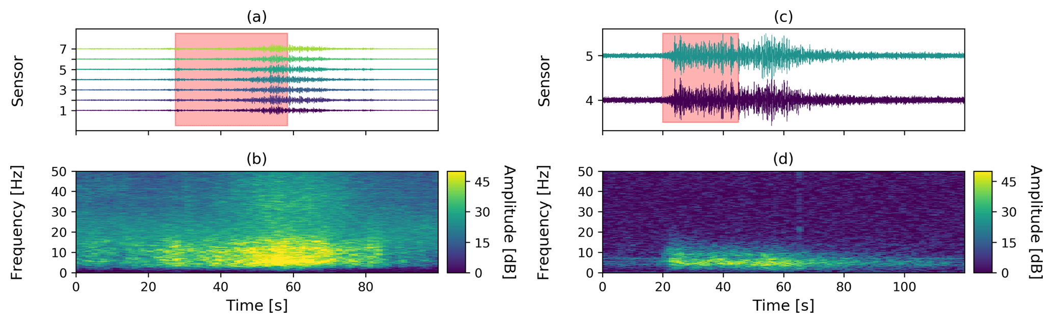
Figure 5An avalanche released on 9 March 2017 at 06:47 LT, and an airplane detected on 28 January 2017 at 09:17 LT used as the training event for the classifier. (a) Time series of the avalanche recorded at the seven sensors of the Dischma array, and (b) time series of the airplane recorded at the two working sensors of the Wannengrat array. The red area indicates the section of the time series used as the training event. (b, d) Corresponding average spectrogram of all sensors.

Download

3.5 Post-processing

As the classification algorithm is not perfect, several post-processing steps were applied to reduce the number of false detections. Detections with a duration ≤12 s were dismissed (Heck et al., 2018), and we only considered an event as an avalanche when it was detected by at least five sensors of the array, as proposed by Heck et al. (2018). Two additional steps were also implemented in the classification workflow and are described in the following.

3.5.1 Combined array detection

Avalanche signals are typically only detected within a radius of 3 km of our seismic arrays (van Herwijnen and Schweizer, 2011b; Heck et al., 2019). As the distance between the Dischma and the Wannengrat array was 14 km, it is very unlikely that an avalanche was recorded at both arrays simultaneously. Thus, signals that were recorded simultaneously at both arrays were most likely not generated by an avalanche. To remove such signals from the events automatically classified at the Dischma array, we implemented a second HMM trained using the airplane event from 31 January at 21:46 LT (Fig. 5b) to classify the data recorded at the Wannengrat and subsequently used the same post-processing steps mentioned earlier. However, as only two sensors recorded data at the Wannengrat array, we only considered events detected by these two sensors. Classification results from the Dischma and Wannengrat arrays were then combined to remove all events recorded simultaneously at both arrays, which meant that the time difference between the detections at both field sites was less than 1 min.

3.5.2 Source localization

Array processing methods provide information on the signal source and can provide additional parameters to classify events as avalanches, as is commonly undertaken when exploiting infrasound signals (Scott et al., 2007; Marchetti et al., 2015; Thüring et al., 2015). To locate the source of events, we used the MUSIC algorithm, as suggested by Heck et al. (2019). The MUSIC method was applied to nonoverlapping data windows for four frequency bands between 6 and 7.5 Hz to determine the back-azimuth angle and the apparent velocity of the incoming wave-field with time. The length of the windows was set to five cycles of the lower corner of the analyzed frequency band, meaning that the data were divided into more windows for higher frequencies. By combining the back-azimuth values for all four frequency bands, we then applied a median smoothing filter on a moving window of 8 s to determine a median back-azimuth path with time, as in Heck et al. (2019) (Fig. 6a).

Figure 6Localization results for an avalanche event recorded on 9 March 2017 at 06:47 LT. (a) Polar plot representation of the back-azimuth calculated using the MUSIC method. Red dots are the back-azimuth values for single time windows. The black line represents the median back-azimuth path. The solid part of the line has variations below the threshold value for the derivative, whereas the dotted line refers to strong variations. (b) The derivative of the median back-azimuth path. The dotted lines represents the threshold value of 10^∘. The section between 52 and 113 s corresponds to the solid line in (a).

Download

To decide whether a classification was associated with an avalanche or not, we applied a threshold value to the derivative of the median back-azimuth path. The assumption was that avalanche events have a relatively smooth median back-azimuth path with little variation, whereas other signal sources show larger variations in back-azimuth, which is also the case for earthquakes and airplanes for our specific array geometry. Indeed, the training event at the Dischma array had a duration of around 50 s and a median back-azimuth path with slight changes in the angle (black line in Fig. 6a), whereas before and after the event the back-azimuths were more erratic, as expected for noise. For the training event, the derivative of the median back-azimuth path stayed below 10^∘ s⁻¹ for 50 s, while before and after the event it was much larger (Fig. 6b). Other avalanche events had very similar results (not shown). Events with derivatives of the median back-azimuth path smaller than 10^∘ for a minimum duration of 20 s were then classified as avalanches. As we used 8 s windows for the calculation of the median back-azimuth path, we had to increase the minimal event duration to 20 s.

We applied our automatic avalanche detection workflow on data recorded at the Dischma field site from 1 January to 30 April 2017. We then compared the results with an avalanche catalogue obtained from visual observations by local observers compiled by the avalanche warning service at the SLF. The visual observations in the Davos area could be incomplete and cover an area much larger than the area monitored with our seismic system at the Dischma site. Nevertheless, comparison with this avalanche catalogue remains indicative.

4.1 Overview of the winter season

The 2016–2017 winter period was relatively short and was characterized by a below-average snow depth. The first snowfalls were quite late in the season, in the middle of December, followed by four weeks with low temperatures and without substantial precipitation. As the thin snowpack was subjected to large temperature gradients for an extended period of time, a poorly bonded layer of depth hoar formed at the base of the snow cover.

During the winter season, four pronounced snowfall periods occurred: between 1 and 15 January, around 1 February, from 1 to 10 March and around 15 April (blue line in Fig. 7). Each snowfall was associated with increased avalanche activity in the Davos region, except for the snowfall in April (red bars in Fig. 7b).

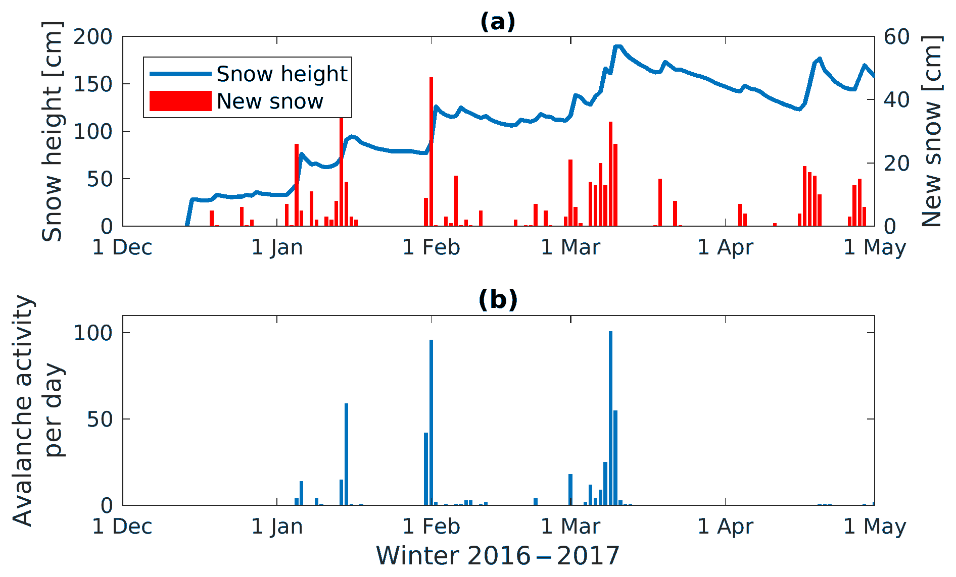
Figure 7(a) Snow height measured (blue line) at the automatic weather station at Weissfluhjoch 12 km to the northwest of the Dischma array at 2540 m a.s.l. for the 2016–2017 winter season. Red bars are the height of new snow measured each day at 08:00 LT. (b) Number of avalanches observed per day in the Davos region (∼175 km²).

Download

In addition to these visual avalanche observations by local observers, we inspected pictures taken by the automatic cameras installed at the Dischma field site. Surprisingly, avalanche activity was very low in January and February, and only a few avalanches were identified on 1 February 2017. During the early March snow storm, visibility was poor and very few avalanches were identified from the automatic camera images. However, once the storm had passed, the intensity of the avalanche cycle became clear as many avalanche deposits were visible on the images. Five days after the storm we mapped 24 avalanches within a 4 km radius of the Dischma field site (for more details see Heck et al., 2019). Later in the season, we did not observe any more avalanches on the images. Thus, the avalanche cycle between 9 and 10 March was the most prominent avalanche period at the Dischma field site.

4.2 Classification performed at a single array

Using the classifier trained using the avalanche event from 9 March 2017 at 06:47 LT (Fig. 5a), we classified the data from each single sensor of the Dischma array and post-processed the results to remove events with a duration ≤12 s and all classifications that were classified by less than five sensors. This resulted in a total of 117 automatically detected events between 1 January and 30 April 2017 (Fig. 8). A quarter of the events were detected by five sensors, a quarter by six and about half by seven sensors.

Figure 8Classification results after post-processing (including voting-based classification) at the Dischma array. The colored bars indicate the number of classified events per day depending on the number of sensors: the violet bar indicates detection by seven sensors, turquoise bars indicate detection by six sensors and yellow bars indicate detection by five sensors.

Download

Most events occurred on 9 and 10 March 2017. In addition, peaks were visible in the middle of January and early April. The peak in January corresponded with the avalanche activity period visually recorded in the Davos region (Fig. 7). For the peak in April, however, no avalanches were observed in the Davos area. Furthermore, several single detections were distributed over the season showing no clear link to the avalanche observations in the Davos region. Therefore, we visually inspected the time series and spectrograms of each of the 117 classifications and found that the HMM also classified ∼50 airplanes (Fig. 9a) and regional earthquakes (Fig. 9b) as avalanches.

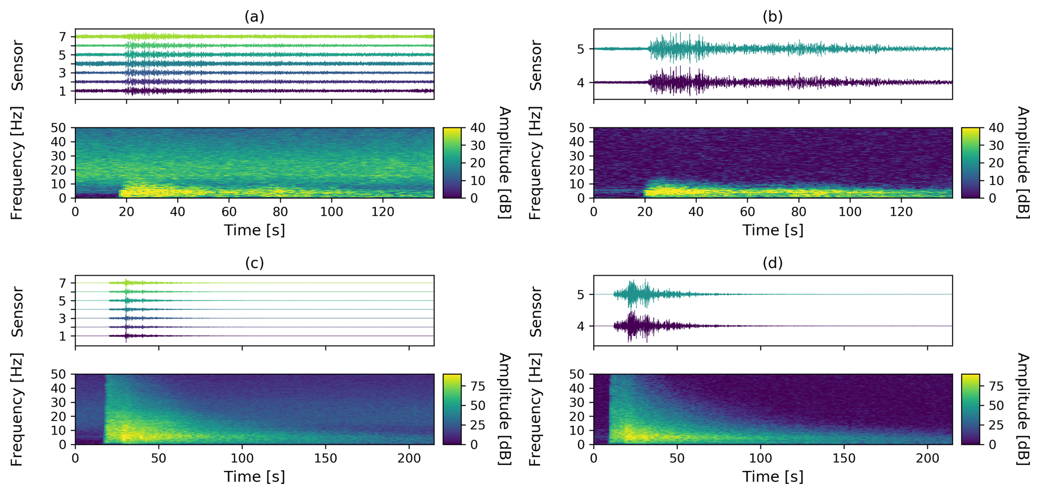
Figure 9Time series and corresponding spectrograms for two false classifications: an airplane detected at (a) Dischma and (b) at Wannengrat, and an earthquake detected at (c) Dischma and (d) Wannengrat.

Download

Although these misclassified events can be distinguished from avalanches via visual inspection (e.g., the sharp onset visible for earthquakes), the classifier identified these events as belonging to the avalanche class. We attribute these false classifications to the fact that these earthquake and airplane signals were more similar to the avalanche training event than to the background model and no earthquake or airplane event type was included in the system. Indeed, the temporal trends in the features exhibited many similarities (Fig. 10). Using different training events did not substantially change these results (not shown).

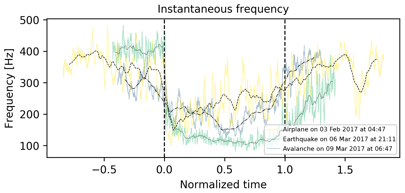
Figure 10Instantaneous frequency with normalized time (normalized with event duration) for signals generated by an airplane (yellow), an earthquake (green) and an avalanche (blue). The black lines are the moving mean. The black vertical dashed lines at zero and one indicate the start and the end of the events.

Download

4.3 Classification performed at both arrays

The vast majority of the misclassifications were produced by two types of events: airplanes and earthquakes. Davos lies in an approach corridor for the Zürich international airport and numerous commercial airplanes pass by every hour. Similar to avalanches, airplanes also have a moving source character. However, due to the high altitude (typically >5 km) and fast movement of the source, airplanes are likely recorded at both arrays. Furthermore, based on the earthquake catalog of the Swiss Seismological Service (SED), we concluded that regional earthquakes within a range of 120 km were recorded by both arrays. Thus, airplanes and earthquakes were recorded almost simultaneously at both arrays (Fig. 9). To eliminate these false classifications, we used data from the Wannengrat array classified using the HMM trained with the airplane event of 31 January at 21:46 LT (Fig. 5b). As the transient signals of airplanes and earthquakes were very similar (Fig. 10), this HMM also detected earthquakes.

The number of detected events at the Wannengrat array varied strongly per day (blue bars in Fig. 11). Fifty-three of these events coincided with events classified at the Dischma array and were dismissed (yellow bars in Fig. 11; Table 1). The remaining 64 potential avalanches were again mostly concentrated in January, around 9 and 10 March and in early April. The distribution of these events was somewhat similar to the visually observed avalanches (compare to red bars in Fig. 7b), except for the detections in April and the absence of detections at the beginning of February. Hence, we expected some misclassifications among the remaining 64 avalanche events.

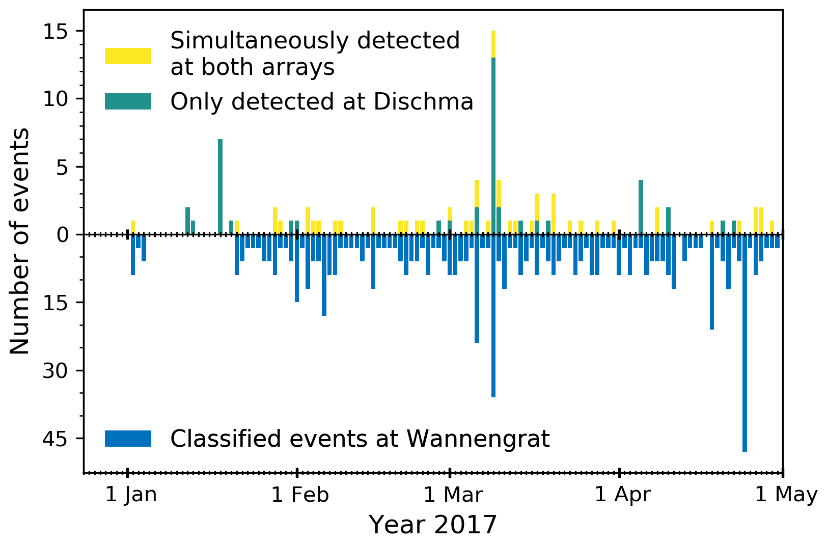
Figure 11Number of events during the season. Yellow bars indicate the events detected at both arrays, turquoise bars show the events only recorded at the Dischma array and blue bars show the events automatically detected at the Wannengrat array. Between 5 and 20 January no data were recorded at the Wannengrat array.

Download

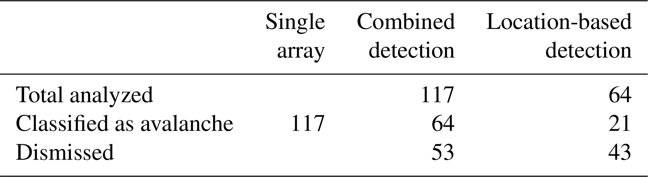
Table 1Number of analyzed events, events classified as an avalanche and dismissed events for the different steps in the classification workflow. For the single array classification, the total number of analyzed and dismissed events cannot be provided as the entire time series was classified.

Download Print Version | Download XLSX

4.4 Localization post-processing

We applied the MUSIC method to the remaining 64 classified events to determine the median back-azimuth paths. Events with derivatives in the median back-azimuth path larger than 10^∘ were dismissed. Following this process, another 43 events were dismissed and only 21 events remained (Fig. 12; Table 1). The majority of these events (i.e., 13 of 21) were observed on 9 and 10 March 2017, whereas the other events showed no clear link to the visual observations (red bars in Fig. 12).

Figure 12Turquoise bars are the number of events per day that are locatable and are considered to be avalanches. Yellow bars are the number of events per day which could not be located and were therefore dismissed. Red bars are the number of avalanches visually observed in the Davos area.

Download

For each of the 21 events we determined a mean back-azimuth, which is the mean direction that the signals came from. The mean back-azimuths were all pointing towards the surrounding slopes where we expected avalanches to release (Fig. 13). Events with a duration longer than 100 s were detected coming from either the northwest or the southeast.

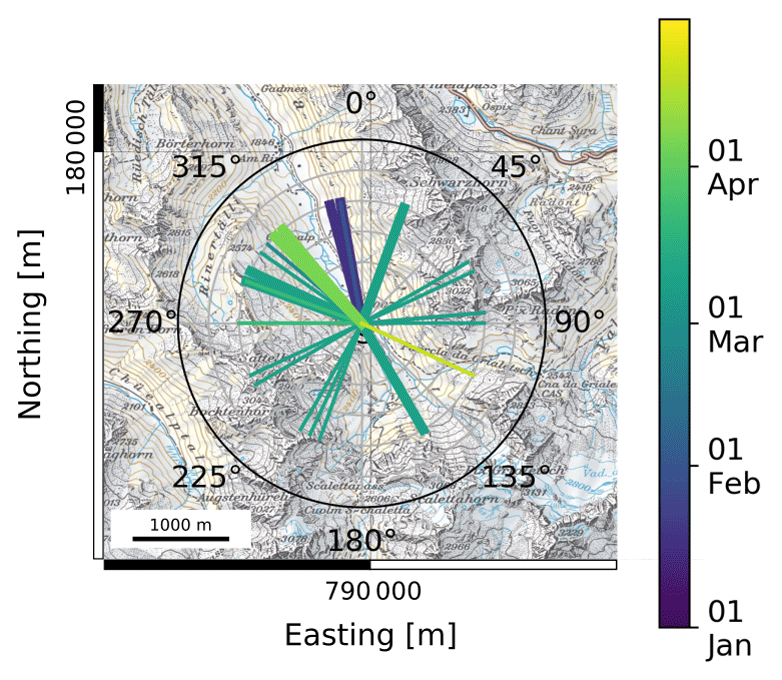
Figure 13Polar plot representation overlaid on a map section of the field site. The angle represents the direction of the origin of the event, the thin lines represent events with a duration <60 s and the thick lines represent events with a duration ≥60 s. The different colored lines represent the time of the year. Reproduced with permission from Swisstopo (JA100118).

Download

Machine learning algorithms are increasingly used for automatic signal detection in seismic data, in particular when investigating gravitational mass movements such as landslides, avalanches, rockfalls and debris flows. They include neural networks (Perol et al., 2018; Esposito et al., 2006), deep learning (Ross et al., 2018), random forest classifiers (Li et al., 2018; Provost et al., 2016), nearest neighbors (Bessason et al., 2007) or kurtosis-based picking (Hibert et al., 2014). While with appropriate calibration these methods generally perform rather well, the main drawback is that a large pre-labeled training database is required. The same is true for signals generated by snow avalanches (e.g., Rubin et al., 2012). The classification workflow we presented used hidden Markov models (HMMs) to automatically detect avalanches in data from seismic systems deployed above Davos, Switzerland. The approach builds on the work of Heck et al. (2018), who adapted the HMM method developed by Hammer et al. (2017) to detect avalanches in continuous seismic data from a small aperture geophone array. A major benefit of this approach is that only one training event is required. This has substantial advantages, as the workflow could be implemented at a newly instrumented site without the need to first establish an extensive training data set. Still, a pre-operational training phase, typically one winter season, is needed to acquire at least one training event and to identify any site-specific peculiarities. Using training events recorded at different arrays might be unreliable due to possible differences in the instrumentation or heterogeneities in the local geology.

For the training event, we only used the first section of the avalanche signal, up to the maximum amplitude (Fig. 5). Using the entire length of the avalanche signal resulted in poorer classification results (not shown) as there were very few variations in the transient feature behavior after the maximum in the signal. Therefore, including larger parts of the training event did not provide any useful additional information for the classification. Heck et al. (2018) also investigated using different avalanche signals to represent different classes (i.e., dry- and wet-snow avalanches). However, this also did not improve the classification results, as in the feature space dry- and wet-snow avalanches are very similar.

Heck et al. (2018) highlighted difficulties involved with obtaining a reliable classifier with the HMM approach applied to a geophone array. They obtained large differences in model performance with the number of detections per sensor ranging from about 150 to over 2000. This was attributed to local heterogeneities as the sensors were packed in a styrofoam housing and inserted within the snow. In our deployment, the geophones were buried about 50 cm below the ground in a flat meadow. This approach resulted in a much more consistent number of detections per sensor, ranging from 125 to 169, showing that the deployment strategy can have substantial influence on the performance of the classifier.

Applying the post-processing steps suggested by Heck et al. (2018) to remove events with a duration ≤12 s and all classifications that were classified by less than five sensors resulted in 117 possible avalanche events (Fig. 8). Even though this approach identified the main avalanche cycle in March 2017 (compare Figs. 7 and 8), visual inspection of the classified events indicated that at least 50 % of the events were generated by airplanes or regional earthquakes (Fig. 9). Although we did not perform an exhaustive sensitivity study, some ad-hoc testing showed that these classification results did not substantially change when training a classifier with different feature combinations, changing the training event and/or changing the length of the training event. The main conclusion to be drawn from this observation is that seismic wave-field attributes of earthquakes and airplanes share significantly more similarities with the seismic wave-field characteristics recorded for avalanches than they do with the characteristics of seismic background noise. In fact, the transient feature behavior of airplanes or regional earthquakes was very similar to signals generated by avalanches (Fig. 10). Thus, implementing an earthquake and airplane HMM at the same site may improve the classification performance. Imposing a duration threshold for the detections did not allow us to detect small avalanches, as signal duration relates to avalanche size (van Herwijnen et al., 2013). However, as powder avalanches travel at higher velocities than wet snow avalanches, it remains unclear what avalanche size is excluded due to the minimum duration threshold. Owing to a lack of ground truth data, we also could not investigate the influence of avalanches size.

To circumvent the problem of developing an optimal event classifier for one specific array, we made use of a second array at the Wannengrat site. There we performed a second classification to automatically identify airplanes and earthquakes using an event model trained using an airplane event. As transient signals produced by earthquakes, airplanes or avalanches have similarities (Fig. 10), the results obtained for the second classification based on the airplane event model likely also include avalanches and earthquakes. However, this was not a drawback as we assume that it was very unlikely that two avalanches released simultaneously at both field sites. Typically, signals generated by airplanes either have clear overtones or at least a clear Doppler effect in the signal (van Herwijnen and Schweizer, 2011a). The airplane signals that were falsely classified as avalanches with our method did not have such obvious features (Fig. 9). While we do not know when or why airplanes generate such signals, and we have not identified a clear pattern explaining their presence, we have seen multiple signals like these recorded at both arrays and are confident that these signals are generated by airplanes. Comparing the time series of detected events at both arrays allowed us to dismiss about 50 % of the classified events (Fig. 11). Therefore, in our case, identifying co-detections across arrays is an efficient approach to reduce the number of false alarms, as the weak signals generated by avalanches were only recorded at one array because the distance between both arrays was about 14 km.

Combining the classification results from two separate arrays allowed us to reduce the number of classifications. Nevertheless, some uncertainty remained regarding the origin of the identified events. Thus, in a final step, we used the MUSIC method to estimate the median back-azimuth path, as suggested by Heck et al. (2019), to further dismiss false detections. Similar approaches have been suggested for the automatic detection of avalanches in infrasonic data by Marchetti et al. (2015) and Thüring et al. (2015). In these studies, the back-azimuth of continuous infrasound data was calculated using cross-correlation techniques, and only events with slight changes in back-azimuth over a predefined minimal duration were assumed to be avalanche events. In contrast, we only determined the back-azimuth using the MUSIC method for those events that were already identified by the HMM, as the pair-wise cross-correlation technique (beam forming) did not result in robust back-azimuth estimates for our instrumentation (Heck et al., 2019). This last processing step further reduced the number of classified events to 21 (Fig. 12).

The majority of the remaining 21 automatic classifications occurred during a period which coincided with the observed high avalanche activity in March (Fig. 12). However, very few avalanches were automatically detected during the first two avalanche periods observed in the area surrounding Davos in January and February. This may be due to the fact that the Dischma site is located about 12 km southeast of Davos where avalanches are regularly observed and weather and snow conditions are sometimes different as major storms arrive from the northwest. Indeed, based on the images from the automatic cameras, very little avalanche activity was observed in the area in January and February, suggesting that there was only one main avalanche period at our site in March. Using our automatic classification results, it was consequently possible to reconstruct the main avalanche activity period in March. Results from the localization showed that avalanches released from many different slopes at the field site during the season, in particular during the avalanche period in March (Fig. 13). Therefore, a seismic monitoring system is a suitable tool to monitor an area with many slopes and not just one single slope. Although the detection range is rather limited at 2–3 km (Heck et al., 2019), the seismic monitoring system in combination with an automatic classifier provide great potential for identifying at least the major avalanche periods. These results suggest that the detection capabilities of seismic monitoring systems are very similar to those of infrasound monitoring systems (Mayer et al., 2018).

Although we were able to identify one major avalanche activity period in the 2016–2017 winter season, the method presented here has its limitations. Our suggested workflow requires two arrays to eliminate events by finding co-detections. This is clearly a limiting factor, as it increases the cost for the instrumentation as well as deployment and maintenance time. However, we could have directly applied the MUSIC method to all detections from the Dischma array to reduce the number of events. Indeed, after applying the localization-based step to all detections, 32 events were identified as avalanches, 11 more than with the combined array and the localization-based classification. Although we decided to implement a combined array classification step to save computational time, directly localizing every automatically detected event is also possible.

The main limitation is that we could not quantify the reliability of the classifier as no independent verification data were available. Our results suggest that the HMMs trained at the Dischma array with a single avalanche training event had a misclassification rate of ∼80 %, which was reduced by applying the suggested post-processing steps. However, the probability of detection or the exact false alarm rate are difficult to estimate, as ground truth data are missing. As avalanches generally release during periods of poor visibility, this is a common problem when assessing the detection performance of automatic avalanche detection systems (Mayer et al., 2018; Heck et al., 2018; Thüring et al., 2015). Alternatively, one could visually inspect the waveforms and spectrograms over the entire season (e.g., van Herwijnen et al., 2016). However, events identified in this manner often contain many uncertainties (Heck et al., 2018). For example, two of the authors independently identified possible avalanches, resulting in 44 and 23 events, respectively. Thus, the only events we could use to assess the performance of our classifier were the 13 manually identified avalanches by Heck et al. (2019) on 9 and 10 March. Twelve of these were automatically identified using our approach, suggesting good performance in terms of the probability of detection and the number of missed events. However, we cannot make any statements regarding the false alarm rate, which from an operational point of view is also very important.

Based on the approach presented here, a near real-time classification of the seismic data and hence a near real-time detection of avalanches seems possible. The computational times on a standard personal computer (with an 8-core processor and 12 GB ram) are reasonably short as feature calculation can be performed in near real-time for all sensors simultaneously as well as the HMM construction and the classification. The MUSIC method, in comparison, is very costly (three times real time). However, as the number of detections for the entire season was very low, a near real-time detection could be provided with or without the combined array classification. In future systems, the preprocessing steps can be integrated in the data logging unit to substantially reduce the data transmission.

The raw seismic data are available upon request. Results from the HMM classification as well as the MUSIC analysis are available at https://doi.org/10.16904/envidat.73 (Heck, 2019).

AvH, JS and DF initiated this study and MH processed and analyzed the data. CH developed the code for the hidden Markov model, and MH developed the code for the MUSIC method. AvH and MH were responsible for the field instrumentation. MH prepared the paper with contributions from all co-authors.

The authors declare that they have no conflict of interest.

This article is part of the special issue “From process to signal – advancing environmental seismology”. It is a result of the EGU Galileo conference, Ohlstadt, Germany, 6–9 June 2017.

This research has been supported by the Schweizerischer Nationalfonds zur Förderung der Wissenschaftlichen Forschung (grant no. 200021_149329).

This paper was edited by Michael Dietze and reviewed by Florian Fuchs and three anonymous referees.