the Creative Commons Attribution 4.0 License.
the Creative Commons Attribution 4.0 License.
 | 22 Jul 2019
Detection and explanation of spatiotemporal patterns in Late Cenozoic palaeoclimate change relevant to Earth surface processes
Sebastian G. Mutz
Todd A. Ehlers
Detecting and explaining differences between palaeoclimates can provide valuable insights for Earth scientists investigating processes that are affected by climate change over geologic time. In this study, we describe and explain spatiotemporal patterns in palaeoclimate change that are relevant to Earth surface scientists. We apply a combination of multivariate cluster and discriminant analysis techniques to a set of high-resolution palaeoclimate simulations. The simulations were conducted with the ECHAM5 climate model and consistent setup. A pre-industrial (PI) climate simulation serves as the control experiment, which is compared to a suite of simulations of Late Cenozoic climates, namely a Mid-Holocene (MH, approximately 6.5 ka), Last Glacial Maximum (LGM, approximately 21 ka) and Pliocene (PLIO, approximately 3 Ma) climate. For each of the study regions (western South America, Europe, South Asia and southern Alaska), differences in climate are subjected to geographical clustering to identify dominant modes of climate change and their spatial extent for each time slice comparison (PI–MH, PI–LGM and PI–PLIO). The selection of climate variables for the cluster analysis is made on the basis of their relevance to Earth surface processes and includes 2 m air temperature, 2 m air temperature amplitude, consecutive freezing days, freeze–thaw days, maximum precipitation, consecutive wet days, consecutive dry days, zonal wind speed and meridional wind speed. We then apply a two-class multivariate discriminant analysis to simulation pairs PI–MH, PI–LGM and PI–PLIO to evaluate and explain the discriminability between climates within each of the anomaly clusters. Changes in ice cover create the most distinct and stable patterns of climate change, and create the best discriminability between climates in western Patagonia. The distinct nature of European palaeoclimates is statistically explained mostly by changes in 2 m air temperature (MH, LGM, PLIO), consecutive freezing days (LGM) and consecutive wet days (PLIO). These factors typically contribute 30 %–50 %, 10 %–40 % and 10 %–30 %, respectively, to climate discriminability. Finally, our results identify regions particularly prone to changes in precipitation-induced erosion and temperature-dependent physical weathering.
- Article
(2679 KB) - Full-text XML
-
Supplement
(1811 KB) - BibTeX
- EndNote


In the study of Earth surface processes, gaining new quantitative understanding of the atmosphere's interaction with the Earth's surface through erosional processes is limited by the difficulty of establishing reliable palaeoclimatic context for erosion rate histories. Such context is particularly useful when erosion rates are calculated using techniques such as cosmogenic radionuclides and low-temperature thermochronology (e.g. Schaller et al., 2002; Bookhagen et al., 2005; Moon et al., 2011; Insel et al., 2010; Stock et al., 2009), which integrate over timescales of 103–106+ years. Despite recognition of the influence of climate on tectonic processes and landscape evolution through erosion (e.g. Whipple, 2009; Montgomery et al., 2001; Willett et al., 2006; Whipple, 2009; Deal et al., 2018), erosion rates calculated from geo- and thermochronological archives are often interpreted under the assumption of modern climate due to insufficient palaeoclimate data (e.g. Starke et al., 2017). While proxy-based palaeoclimate reconstructions, or reconstructions of climate-controlled variables such as river discharge (e.g. Wickert, 2016), are in some cases able to provide sufficient and plausible context for specific problems, general circulation models (GCMs) offer a complementary and integrative approach to palaeoclimate reconstructions. GCMs complement proxy-based reconstructions in several ways: (1) GCMs have a global coverage (e.g. Salzmann et al., 2011; Haywood et al., 2013; Jeffrey et al., 2013) and therefore provide palaeoclimatological context in regions with sparse proxy records; (2) GCM-based palaeoclimate reconstructions allow the refinement of local proxy-based reconstructions by providing regional means and a broader climatic context; (3) GCMs are able to offer insight into atmospheric drivers of reconstructed local palaeoclimates, because they simulate atmospheric processes based on our physical understanding of the climate system; (4) GCMs allow the conduction of sensitivity experiments to investigate the relationship between climatic drivers and local observations (e.g. Takahashi and Battisti, 2007).
The Paleoclimate Modelling Intercomparison Project (PMIP) coordinates palaeoclimate modelling efforts (Kageyama et al., 2018) and provides experiment designs for the Mid-Holocene and the last interglacial (Otto-Bliesner et al., 2017), the last millennium (Jungclaus et al., 2010), the Last Glacial Maximum (Kageyama et al., 2017), and the Pliocene Warm Period (Haywood et al., 2016), which is part of the Pliocene Model Intercomparison Project (PlioMIP). Despite consistent forcings, experiments carried out with different GCMs and model resolutions yield different results due to GCM specific parameterisation. Mutz et al. (2018) conducted PMIP-style palaeoclimate experiments with the same GCM (ECHAM5) and resolution, which removes the GCM parameterisation related signal in the differences between simulated palaeoclimates. This experiment framework comprises climate simulations for the pre-industrial (PI, reference year 1850), Mid-Holocene (MH, ∼6 ka), Last Glacial Maximum (LGM, ∼21 ka) and Pliocene (PLIO, ∼3 Ma).
This study takes advantage of the Mutz et al. (2018) simulation framework and quantifies differences between simulated palaeoclimates with regard to variables relevant to Earth surface processes (e.g. rainfall characteristics, temperature-derived quantities, wind speed and direction) in order to allow more refined interpretations of potential climatic drivers for changing rates in Earth surface processes. For more effective communication of our methods and results, we separate the PI control simulation from MH, LGM and PLIO in discussion by referring only to the latter three as Late Cenozoic climates. These are time periods over which reconstructed erosion rates typically integrate. Understanding how different these palaeoclimates are from a pre-industrial climate with regard to variables that potentially affect erosion rates is essential in any comprehensive and merited interpretation of erosion rates, and ultimately allows for better assessment of the influence of climatic and tectonic controls on erosion. Three questions are addressed in this study:
-
What are the spatial patterns of climate change in comparisons of pre-industrial with Late Cenozoic time periods?
-
How different were Late Cenozoic palaeoclimates from the pre-industrial climate with regard to variables relevant to Earth surface processes?
-
What constitutes these quantified differences between pre-industrial and Late Cenozoic climates?
We focus on four regions that are frequently investigated with regard to erosion histories: southern Alaska, western South America, South Asia and Europe. The first question is addressed by conducting a cluster analysis of the differences between pre-industrial and Late Cenozoic palaeoclimates, which subdivides the four study regions into geographical clusters governed by a distinct character of erosion-relevant climate change. Whereas Mutz et al. (2018) apply a similar cluster analysis to describe the modes of climate variability in each palaeoclimate simulation, the results of this study consist of maps showing the extent of a particular mode of climate change and thus provide an overview of climate change over time. The resulting clusters also serve as suitable masks for values used in the discriminant analyses. Questions 2 and 3 are addressed by conducting discriminant analyses of subdivisions of the four study areas, which are objectively predefined by the aforementioned cluster analyses. The results provide a quantitative assessment and explanation of differences in climate with regard to variables relevant to Earth surface processes.
The overarching goal is to provide the Earth surface science community with an overview and quantitative assessment and explanation of how climate changed in the Late Cenozoic with regard to variables relevant to Earth surface processes. However, the same methods may also be applied to simulations of modern and future climates to detect and explain patterns of climate change that may result in shifts of Earth surface process regimes.
This section describes the data, methods and processing steps. In summary, we apply a cluster analysis that identifies where surface-process-relevant aspects of climate change are likely and a discriminant analysis that quantifies and explains these changes within the regions identified by clustering. This combination of clustering and discrimination of climate model simulation results yields five different sets of results (Fig. 1): anomaly maps for a set of climate variables (in the Supplement to this paper), multivariate anomaly cluster maps and anomaly cluster characterisations (Sect. 2.2), discrimination scores and a measure of relative contribution by each climate variable to discriminability (Sect. 2.3). While the individual components of the processing chain (Fig. 1) are based on well-established methods, the processing setup and the particular combination of these methods is tailored to address this study's specific scientific problems.
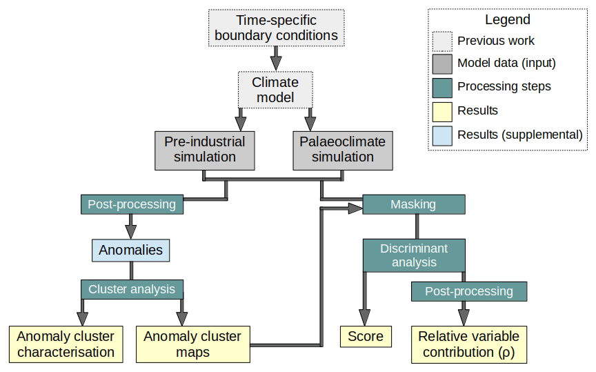
Figure 1Anomalies are created from pre-industrial (PI) and Late Cenozoic palaeoclimates (MH, LGM, PLIO). These are subjected to geographical clustering, which results in the identification of distinct modes of climate change (anomaly cluster characterisation) and maps showing the spatial extent of regions governed by these modes (anomaly cluster maps). These are used as geographical masks for palaeoclimate simulations. For each of these anomaly clusters, a discriminant analysis is conducted to quantify the discriminability in each cluster (score) and the relative contribution of each climatic variable to this discriminability.
2.1 ECHAM5 simulations
GCMs simulate global climate based on our physical understanding of atmospheric processes and are primarily used to investigate atmospheric dynamics and contemporary climate change but have also been applied to improve our understanding of past climates and Earth system dynamics (e.g. Kutzbach et al., 1993; Ehlers and Poulsen, 2009; Maroon et al., 2015, 2016; Mutz et al., 2016, 2018). GCMs have become well-established tools in geoscience, as is reflected by the work of the PMIP (Kageyama et al., 2018; Bracannot et al., 2012), which adds palaeoclimate-related contributions to the Coupled Model Intercomparison Project (CMIP). Palaeoclimate studies address a range of different timescales including the last millennium (e.g. Jungclaus et al., 2010), orbital (e.g. Gong et al., 2013; Lohmann et al., 2013; Pfeiffer and Lohmann, 2016; Wei and Lohmann, 2012; Zhang et al., 2014) and tectonic timescales (e.g. Knorr et al., 2011; Stepanek and Lohmann, 2012). Comparisons between palaeoclimate simulations of different time periods are often complicated by use of different models and inconsistencies in model setup. Parameterisations specific to individual GCMs and differences in horizontal and vertical resolution introduce differences between simulations that are not a result of prescribed forcings.
Mutz et al. (2018) conducted a suite of GCM simulations conducted with the same GCM (ECHAM5) and resolution to circumvent the above-mentioned biases. This GCM simulation framework comprises palaeoclimate experiments for pre-industrial times (reference year 1850), the Mid-Holocene (approximately 6.5 ka), the Last Glacial Maximum (approximately 21 ka) and the Pliocene (approximately 3 Ma) climates. The experiments were conducted at a spectral resolution of T159 (approximately 80 km ×80 km), with 31 vertical levels and an output frequency of 1 d. The simulations are based on boundary conditions from coupled atmosphere–ocean coupled general circulation model (AOGCM) transient simulations and palaeoenvironmental reconstruction initiatives such as PMIP3 (Abe-Ouchi et al., 2015), GLAMAP (Sarnthein et al., 2003), CLIMAP (CLIMAP project members, 1981), PRISM (Haywood et al., 2010; Sohl et al., 2009; Dowsett et al., 2010) and BIOME6000 (Prentice et al., 2000; Harrison et al., 2001; Bigelow et al., 2003; Pickett et al., 2004). For a detailed description of model setups, we refer the reader to Mutz et al. (2018) and references therein.
The high resolution and model consistency across all of the time slice experiments in the Mutz et al. (2018) climate simulation set has not been achieved previously in the palaeoclimate modelling community. These GCM experiments therefore represent a unique, state-of-the-art simulation framework suited for investigations of changes in climate-controlled processes across the Late Cenozoic. The GCM (ECHAM5) is a well-established model in the climate community, and simulated palaeoclimates are in agreement with other modelling and proxy-based reconstruction efforts. Mutz et al. (2018) use a present-day simulation to establish confidence in the model and compare palaeoclimate estimates to compilations of proxy-based reconstructions for MH and LGM precipitation over South America and Tibet. The proxy comparisons reveal a satisfactory to good performance of the GCM, thus highlighting the suitability of GCMs in the study of palaeoclimate-related problems. The latitudinal gradients and magnitude of difference in temperature and precipitation are in good agreement with results of previous palaeoclimate modelling efforts. We refer the reader to Mutz et al. (2018) for a detailed comparison to other palaeoclimate simulations and proxy-based reconstructions.
2.2 Clustering – multivariate anomaly maps
This study's investigation of differences focusses on four regions, which (a) are of interest to the Earth surface and palaeo-altimetry communities, and (b) are feasible to work on given the GCM's limitations (see Mutz et al., 2018): southern Alaska (52–68∘ N, 125–165∘ W), western South America (5–56∘ S, 60–80∘ W), Europe (26–65∘ N, 22∘ W–66∘ E) and the South Asia (0–60∘ N, 40–120∘ E). Climate change within each of the investigated region is spatially heterogenous in both direction and magnitude (Mutz et al., 2018). In the example of PI–LGM climate change in Europe, southern Norway experiences a strong increase in consecutive freezing days and strong decrease in 2 m air temperature, while continental Europe experiences only mild cooling but strong increases in intra-monthly 2 m air temperature variability. We refer to these combinations of changing climate attributes as “modes of (climate) change” in this paper. Each of the regions is governed by a number of these distinct modes of climate change. These intra-regional discrepancies merit an informed and objective subdivision of each region into geographical subdomains governed by one of these modes of change prior to the investigation of differences in climate through time. Geographical clustering allows such subdivisions on the basis of similarities in climate change at different locations within each region. It assesses climate change for each grid box, calculates its similarity to climate change in other grid boxes and groups them accordingly. More specifically, it allows the grouping of elements (i), in this case climate model surface grid boxes, by the co-variability of anomalies of selected climatic element attributes. For each region, the contained elements are subjected to agglomerative hierarchical clustering, followed by k-means clustering corrections (Mutz et al., 2016; Paeth, 2004) to address the inherent shortcomings of a pure hierarchical approach. The Mahalanobis distance (e.g. Wilks, 2011) is used as a measure of similarity (of climate change) between clusters in the entire procedure. Readers are referred to Mutz et al. (2018) for a more detailed description of the procedure and aforementioned shortcomings.
Table 1Code, units, explanation and geomorphic relevance of each of the climate attribute variables used in the cluster and discriminant analysis.
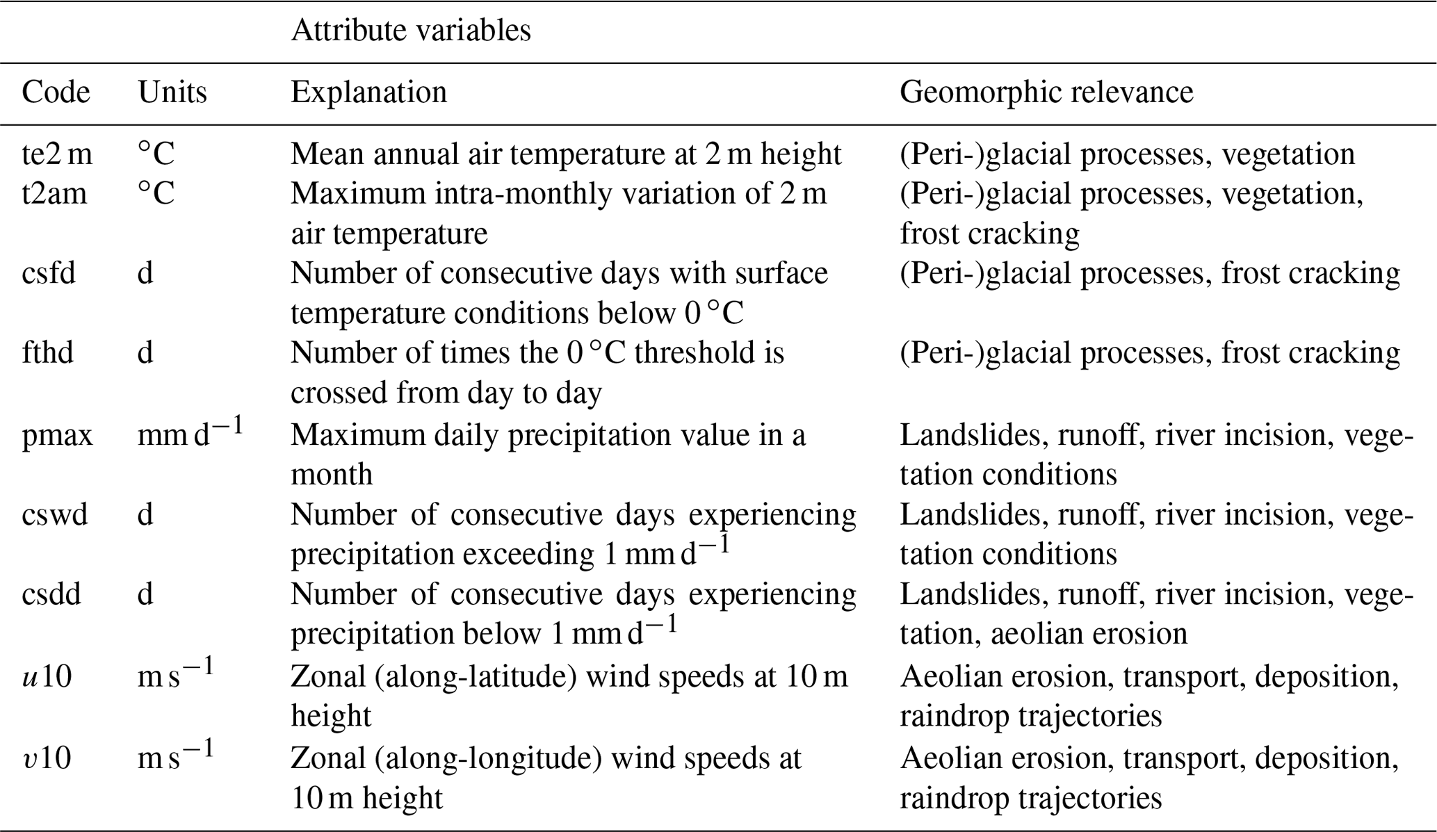
The clustering is conducted on basis of the same climatic attributes as the discrimination between climates through time (Sect. 2.3). In total, M (=9) element attributes, summarised in Table 1, are chosen based on (1) their relevance to Earth surface processes, (2) their adequate representation by the GCM and (3) the feasibility of construction from GCM output: near-surface air temperature (te2 m), intra-monthly near-surface air temperature amplitude (t2am), consecutive freezing days (csfd), freeze–thaw days (fthd), maximum precipitation (pmax), consecutive wet days (cswd), consecutive dry days (csdd), zonal near-surface wind speeds (u10) and meridional near-surface wind speeds (v10).
For calculation of consecutive freezing days and freeze–thaw days, a surface temperature of 0 ∘C is taken as a threshold value. The maximum duration of a wet period, i.e. precipitation exceeding 1 mm d−1 (Zolina et al., 2010; Zhang et al., 2011) constitutes the cswd attribute. Inversely, the maximum duration of a dry period, i.e. precipitation failing to exceed the 1 mm d−1 threshold (Zin and Jemain, 2010), constitutes the csdd attribute. These attribute variables are constructed from each palaeoclimate (MH, LGM and PLIO) and reference simulation (PI) output. The climate attribute anomalies, which serve as a basis for the clustering, are then calculated for time slice comparisons PI–MH, PI–LGM and PI–PLIO.
Clustering requires an a priori decision on the number of clusters (k) or subdivisions per region. The optimal value of k is not known before clustering. Therefore, k is varied in our experiments, and the cut-off point for the parameter is set once the increase in k no longer results in a cluster with distinct climatic character but instead results in a weakened or strengthened character of an already existing cluster. Since optimal k can be expected to roughly scale with region size, the parameter is varied from 3 to 5 for southern Alaska and from 5 to 8 for the larger regions. The results consist of optimal geographical subdivisions (climate clusters C1–Ck) with distinct climatic characters, which are described by mean vectors for climate attribute anomalies. Every cluster-characterising vector has a length of M. For each of the time slice comparisons and clusters, the discriminability and relative contribution to it by each of the M attribute variables is quantified in the procedure described in Sect. 2.3.
2.3 Discrimination – quantifying and explaining anomalies
The multivariate linear discriminant analysis (LMD) (e.g. Wilks, 2011) is a statistical tool that allows the investigation and explanation of differences between two or more groups with regard to multiple attribute variables. More specifically, it quantifies the discriminability of the groups and the contribution of each of the attribute variables to this discriminability. The resulting discrimination model can be applied to objectively categorise an element with unknown group affiliation. In this study, the time periods (PI, LGM, MH and PLIO) are used as groups, and the aforementioned climate variables relevant to Earth surface processes are chosen as group attributes. Since the focus of this study lies on the assessment of the differences between two specific time periods with regard to multiple climate variables, the problem is treated as a two-group multivariate case.
The centre piece of the analysis lies in finding a discriminant function that best separates the two groups (or palaeoclimate time slices). This is carried out for each comparison, i.e. each pair of palaeoclimate time slices. This discriminant function can be expressed as a linear combination of the climate attribute variables:
where Y is the discriminant function, Xm (m=1…M) are the climate variables used to assess the differences in palaeoclimates, υm (m=1…M) is the discriminant coefficients associated with each variable. υ0 is a constant (the y intercept) that is of no relevance to the goodness of separation and will therefore no longer be mentioned. In this case, M=9 (te2 m, t2am, csfd, fthd, pmax, cswd, csdd, u10, v10). Each climate variable Xm (see Table 1) contains elements xmn (n=1…N), where N is the number of elements in each cluster. Each element (or grid box) is associated with a discriminant value (yn) described by
In other words, the elements yn (n=1…N) are projected onto the discriminant axis Y. The problem of finding a discriminant function that best separates the two groups (or palaeoclimates) can therefore also be seen as the process of finding an axis on which the frequency distributions of the projected elements yn for the two groups show the smallest overlap. Since overlap is a function of distance between groups (D) as well as the scatter within them (S), the difference between these frequency distributions is described by the distance between the two group centroids (i.e. the group means of the projected elements yn on the discriminant axis) and the scatter within the group (i.e. sum of squared deviations from the means). This distance, i.e. the discriminant criterion Γ, is maximised in order to find the best discriminant function Y and corresponding discriminant coefficients υm (m=1…M). The problem in the two-group multivariate case of this study can thus be summarised as
Γ is the discriminant criterion, T1 and T2 are the two groups (e.g. PI and LGM in the case of time slice comparison PI–LGM), and nT1 and nT2 are the number of elements in T1 and T2. We can express the discriminant function as a matrix calculation:
where
and solve the above-mentioned optimisation problem via partial derivatives with respect to the discriminant coefficients (υ) (e.g. Wilks, 2011). The discriminant coefficients are then standardised, i.e. put in relation to the standard deviations of respective variables, to yield ω. The relative contribution (ρ) of each of the M attribute variables to discriminability is calculated as
Finally, the skill of the resulting discrimination model is evaluated. For this, the association of each element to groups T1 (PI) or T2 (MH, LGM or PLIO) is forgotten, and the elements are re-categorised according to the critical discriminant values of the models (e.g. Bahrenberg et al., 1992). The fraction of correct classifications (the score) is calculated and used as a measure of “goodness of separation” given by the models. The described LMD procedure is applied to each time slice comparison of T1-T2 (namely PI–MH, PI–LGM and PI–PLIO) and each of the k climate anomaly clusters (C1, C2, …, Ck) in the four study regions. Each calculation yields two variables suitable for addressing the problems treated in this study: (1) a measure for goodness of discriminability (score) and (2) a measure for the relative contribution (ρ) of each of the M attribute variables to discriminability. A maximum score of 1 indicates perfect separation of all values, whereas a score of 0 indicates that the discrimination model has no explanatory power at all. Attribute variables associated with a ρ value of 1 are solely responsible for the discrimination, whereas those associated with a ρ value of 0 contribute nothing to the discriminability between climates.
2.4 Example problem
In summary, the clustering of anomalies (Sect. 2.2) reveals geographical clusters (or subdivisions in each of the study regions), in which similar climate change occurs, and describes the mode of climate change in each of these clusters. The LMD (Sect. 2.3) then quantifies the discriminability of climates in these clusters and explains it with the climatic attribute variables. The set of results for each time slice comparison and region therefore consists of four components: (1) anomaly (cluster) maps that show the spatial extent of dominant modes of climate change; (2) anomaly cluster characterisation that consists of mean vectors of climate change within each cluster and describe the mode of climate change experienced in the grid boxes assigned to the same cluster; (3) discrimination scores that describe the goodness of discriminability of climates within each of the anomaly clusters; and (4) relative variable contribution, which describes the contribution of each of the climatic attribute variables to the discriminability calculated for each of the anomaly clusters. How these sets of results may be used in answering questions pertaining to climate-driven Earth surface processes is demonstrated in the simplified example below.
Erosion rates were calculated, for example, by means of cosmogenic nuclides, for a region in a specific area of interest circled on the map (Fig. 2). Although they are taken as modern (time T1) erosion rates, the signal integrates over 10 000 years and includes erosion rates at time T2. In order to find out if and how significantly erosion rates may actually have been different at time T2, Fig. 2 is consulted.

Figure 2Example problem: investigating how climatic boundary conditions for erosion processes have changed in a specific region of interest involves consultation of part of the conceptualised results figure. The location of the region of interest geographically coincides with the region assigned to cluster C1. Consequently, only the results related to C1 are consulted and the rest is greyed out. The clusters were calculated from the differences in the values (delta values) of geomorphically relevant climate variables between two different times (T1 and T2) in the Late Cenozoic and thus represent a specific mode of change. The mode of change associated with the cluster of interest (C1) is revealed by the purple–green column. The relative contributions of the delta values to the overall discriminability between T1 and T2 in cluster C1, indicated by the score, is revealed by the diameters of the circle superimposed onto the delta values in the purple–green column.
The anomaly cluster map shows the large-scale spatial patterns of changes in climatic variables relevant to Earth surface processes. Each cluster is associated with a specific mode of climate change, and all locations that fall within it experience this type of climate change. The area of interest lies in cluster C1, so all information not related to C1 and the area of interest is shaded in pale grey to remove distractions. The purple–green raster plots reveal the type of climate change associated with C1 and thus with the circled area of interest: T2 had a little more rainfall, a lot more (consecutive) wet days, higher temperatures, fewer freezing days and fewer (consecutive) dry days. Does the climate of T2 have a distinct enough signature to tell it apart from T1? The score is reasonably high, which reveals that the climate of T2 does indeed have a distinct signature and consequently, it suggests a good possibility for a different erosional regime or erosive intensity.
In order to assess the consequences of the mode of climate change in C1 for erosion, the circles (Fig. 2) are examined. Those explain which anomaly of which variable is responsible for the distinct signature that has been detected and described above. They indicate that approximately 60 % of this “discriminability” can be explained by increases in temperature and approximately 40 % by increases in consecutive wet days. Consequently, it is reasonable to assume a priori that erosive processes controlled by these parameters may be affected significantly. The specific sensitivity of conditions and processes at the Earth's surface, e.g. vegetation or critical thresholds in landscape responses, cannot be taken into consideration in these results due to the highly variable nature of them. However, the exact magnitudes of those significant (and insignificant) changes are listed in Table S1 in the Supplement to allow the reader to assess the specifics of the impact of climate on processes of the specific area and problem at hand. The above example provides the basic concepts needed to understand the remaining figures in this paper.
This section contains descriptions of results from the cluster and discriminant analyses carried out for each of the time slice comparisons and study regions. It is divided into sections for the three major study regions: Sect. 3.1 (western South America), Sect. 3.2 (Europe) and Sect. 3.3 (South Asia). For brevity, the results for southern Alaska are included in the Supplement (Fig. S10). For each subsection, regional results for time slice comparisons PI–MH, PI–LGM and PI–PLIO are presented. The figures accompanying each of those consists of four elements (see Sect. 2.4): (1) the first element to the figures are multivariate anomaly maps that were created by clustering the differences between climatic attribute variables in each of these comparisons (see Sect. 2.2) and show the resulting geographical subdivision into clusters governed by a specific mode of climate change. (2) The second element to the figures is (purple and green) raster plots showing the characterisation of those clusters. They describe the mode of change, i.e. the magnitude and direction of changes observed on average in each of the clusters. For visual clarity, the magnitude of change is scaled by the maximum absolute difference in each region and time slice comparison. Numerical values are listed in tabular format in the Supplement to this paper (Table S1). (3) The third (grey) element consists of the scores for each cluster. These are based on a discriminant analysis carried out for the cluster (see Sect. 2.3) and describe the goodness of discriminability of the palaeoclimates in comparison to the PI control simulation. (4) The fourth and final element to the figures consists of a measure for the relative contribution (ρ) of each of the nine climate variables (Table 1) to the overall discriminability between two time slices in each geographical cluster. This element is displayed as a layer of circles on top of element 2 and reveals how much an anomaly of a specific variable (represented by a specific shade of purple or green) contributes to the discriminability between PI and a palaeoclimate in each of the clusters. Larger circle diameters correspond to greater contributions.
For brevity, results for these time slice comparisons (PI–MH, PI–LGM and PI–PLIO) are simply referred to as results for MH, LGM and PLIO, respectively. The notations MH-Ci, LGM-Ci and PLIO-Ci are used to refer to results for the ith geographical subdivision (or cluster) in the respective set of results. Descriptions of changes in climate are implicitly discussed in the context of the control simulation and are therefore descriptions of deviations from the PI climate. Discussions of multivariate anomaly maps and cluster characterisation (elements 1 and 2) focus mostly on the stable and persistent patterns seen in the results, i.e. geographical clusters that are least sensitive to changes in k and keep their distinct character. Discussions of scores and relative contribution to discriminability (ρ) focus primarily on clusters with good discriminability. Additional information on climate change on a sub-cluster scale are given in the form of single-variable anomaly maps in the Supplement to this paper (Figs. S1–S9).
3.1 Western South America
3.1.1 Large-scale patterns and modes of climate change
In western South America, the dominant modes of change for the MH are captured in clusters MH-C3, MH-C4, MH-C5 and MH-C6 (Fig. 3a, d). MH-C3 covers much of central Patagonia and is characterised by decreases in consecutive freeze–thaw days and increases in consecutive freezing days and consecutive wet days. MH-C4 is the mode of change observed in most of Argentina and the central and southern Andes. It consists of relatively small increases in consecutive wet days and freeze–thaw days. MH-C5 covers most of the tropics in the region and is characterised by decreases in consecutive wet days and maximum precipitation, and relatively small increases in 2 m air temperature and consecutive dry days. Relatively large increases in 2 m air temperature and consecutive dry days, and decreases in maximum precipitation and consecutive wet days constitute the mode of change for MH-C6, which extends over low-altitude subtropics in the region.
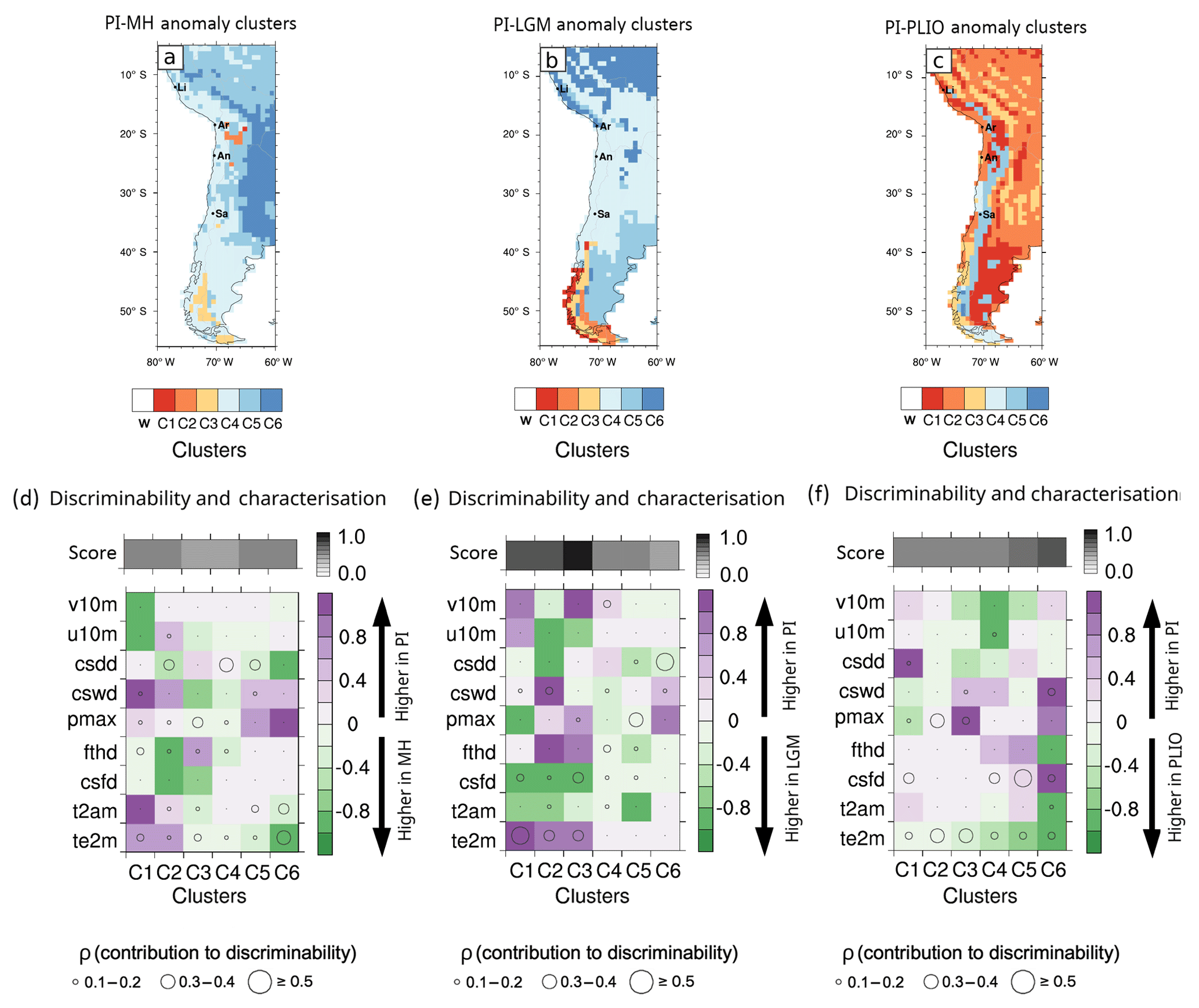
Figure 3The multivariate anomaly maps for time slice comparisons PI–MH (a), PI–LGM (b) and PI–PLIO (c) show the geographical coverage of clusters C1–Ci in western South America, which describe the spatial extent of regions characterised by similar modes of change. The corresponding modes of change (d, e, f) for each cluster are expressed as relative changes in each of the nine investigated variables (Table 1): 2 m air temperature (te2 m), 2 m air temperature amplitude (t2am), consecutive freezing days (csfd), freeze–thaw days (fthd), maximum precipitation (pmax), consecutive wet days (cswd), consecutive dry days (csdd), zonal near-surface wind speeds (u10) and meridional near-surface wind speeds (v10). The score (d, e, f) expresses the goodness of discriminability between palaeoclimate pairs PI–MH (d), PI–LGM (e) and PI–PLIO (f) in each of the anomaly clusters. The size of the circles corresponds to the relative contribution of each of the nine climatic attribute variables to the measured discriminability in each anomaly cluster for all three time slice comparisons.
LGM-C1–LGM-C3 share a number of characteristics. These modes of changes include decreases and 2 m air temperature and increases in 2 m air temperature amplitude and consecutive freezing days (Fig. 3e). Furthermore, the region occupied by LGM-C1–LGM-C3 is covered by ice in the LGM. Differences between these modes of changes include a large increase in maximum precipitation in LGM-C1 and decreases in consecutive wet days in LGM-C2. LGM-C4, covering much of the subtropics in the region, is characterised by relatively little change in all of the investigated variables. LGM-C5 covers much of eastern Argentina and experiences increases in 2 m air temperature amplitude. LGM-C6 covers much of the tropics of the region and is characterised primarily by decreases in maximum precipitation and consecutive wet days.
The dominant modes of change in the PLIO are described by PLIO-C1, PLIO-C2, PLIO-C3 and PLIO-C5 (Fig. 3f). Covering much of eastern Argentina and parts of the central Andes, PLIO-C1 is characterised primarily by relatively large decreases in consecutive dry days and increases in maximum precipitation and consecutive wet days. The grid boxes assigned to PLIO-C2, extending over most of the low-altitude tropics and subtropics and the Atacama Desert, experience very little change on average. For grid boxes assigned to PLIO-C3, a decrease in maximum precipitation and consecutive wet days, and increase in consecutive dry days and meridional wind speeds can be observed. PLIO-C5 extends over much of the central and southern Andes and is characterised by decreases in freeze–thaw days and increases in 2 m air temperature and meridional wind speeds. While PLIO-C6 experiences some of the largest changes, it only covers the Northern and Southern Patagonian ice fields and coincides with the reduction of the ice cover in the PLIO simulation.
3.1.2 Discriminability
The discrimination scores (Fig. 3d, e, f) are highest for the LGM and lowest for the MH, and changes in temperature, consecutive freezing days, maximum precipitation and consecutive dry days are factors that explain much of the discriminability overall. LGM-C1–LGM-C3 s have the highest scores. In all three clusters, decreases in 2 m air temperature are one of the primary contributors to the discriminability between LGM and PI climate. They explain 40 %–50 % of the discriminability in LGM-C1 and 30 %–40 % in LGM-C2 and LGM-C3. With 20 %–30 % explained discriminability in LGM-C1 and 30 %–40 % explained discriminability in LGM-C3, increases in consecutive freezing days are a second important factor for discriminability between the climates in western Patagonia. Discrimination with PLIO and PI simulations yields the highest scores for PLIO-C6, which covers the Patagonian Ice Fields, and PLIO-C5. Increases in 2 m air temperatures and decreases in consecutive wet days and consecutive dry days explain the discriminability in PLIO-C6 in equal parts (20 %–30 %). An increase in temperatures and relatively small decrease in consecutive freezing days explain 20 %–30 % and 40 %–50 % of the discriminability in PLIO-C5, respectively.
3.2 Europe
3.2.1 Large-scale patterns and modes of climate change
MH-C1 covers Spain and the region east of the Caspian Sea (Fig. 4a) and is associated with the least change in climate attribute variables. MH-C2, covering areas in western Europe, western Russia and the Mediterranean coasts (Fig. 4a), experiences an increase in maximum precipitation (Fig. 4d). Ukraine, Poland, much of the Baltic Sea coast and southern Scandinavia are assigned to MH-C3 and experience decreases in freeze–thaw days. MH-C4 and MH-C5 primarily cover northern Africa and are characterised by increases in 2 m air temperature and maximum precipitation.
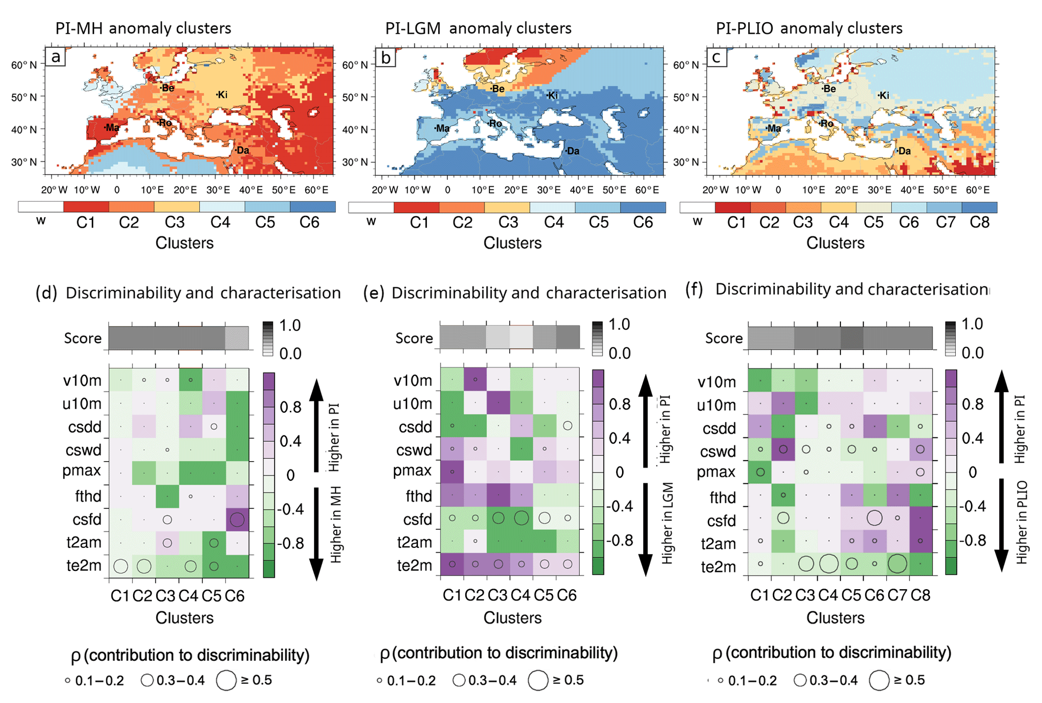
Figure 4The multivariate anomaly maps for time slice comparisons PI–MH (a), PI–LGM (b) and PI–PLIO (c) show the geographical coverage of clusters C1–Ci in Europe, which describe the spatial extent of regions characterised by similar modes of change. The corresponding modes of change (d, e, f) for each cluster are expressed as relative changes in each of the nine investigated variables (Table 1): 2 m air temperature (te2 m), 2 m air temperature amplitude (t2am), consecutive freezing days (csfd), freeze–thaw days (fthd), maximum precipitation (pmax), consecutive wet days (cswd), consecutive dry days (csdd), zonal near-surface wind speeds (u10) and meridional near-surface wind speeds (v10). The score (d, e, f) expresses the goodness of discriminability between the palaeoclimate pairs PI–MH (d), PI–LGM (e) and PI–PLIO (f) in each of the anomaly clusters. The size of the circles corresponds to the relative contribution of each of the nine climatic attribute variables to the measured discriminability in each anomaly cluster for all three time slice comparisons.
LGM-C1–LGM-C4 (Fig. 4b) are all partially characterised by a decrease in 2 m air temperature and freeze–thaw days, and increases in consecutive freezing days (Fig. 4e). It should be noted that grid boxes assigned to these clusters are covered by the Fennoscandian and British ice sheets in the LGM simulation. LGM-C5 extends over much of the Mediterranean region, Spain and European north Russia, and is characterised by increases in 2 m air temperature amplitude, consecutive dry days and relatively small increases in freeze–thaw days and decreases in maximum precipitation and consecutive wet days. Most of central Europe, western Asia and north Africa is assigned to cluster LGM-C6 and experiences the least change.
The dominant modes of change in the PLIO are captured in PLIO-C3–PLIO-C6 (Fig. 4c). PLIO-C3 is a mode of change mostly seen in parts of north Africa and characterised by increases in meridional and zonal wind speeds (Fig. 4f). In the coastal regions north of it, very little change is seen in the PLIO (PLIO-C4). PLIO-C5 covers much of central Europe and experiences decreases in freeze–thaw days and 2 m air temperature amplitude, and relatively small increases in 2 m air temperature. European Russia and parts of Scandinavia are assigned to PLIO-C6 and experience increases in freeze–thaw days and 2 m air temperature, and decreases in consecutive dry days and 2 m air temperature amplitude. PLIO-C7 is mostly distributed along parts of the Mediterranean, Black Sea and Caspian Sea coasts and characterised by increases in consecutive dry days and 2 m air temperature, and a decrease in freeze–thaw days. PLIO-C8 covers southeastern Norway and the Alps and is characterised by decreases in consecutive freezing days and 2 m air temperature amplitude, and increases in 2 m air temperature and freeze–thaw days.
3.2.2 Discriminability
In all time slice comparisons, changes in 2 m air temperature explain most of the discriminability in many of the geographical clusters (Fig. 4d, e, f). Changes in consecutive freezing days and consecutive wet days are also major contributors to discriminability in the LGM and PLIO, respectively. LGM-C1 , LGM-C2, LGM-C5 and LGM-C6 are associated with the highest scores for the LGM. Overall, 20 %–24 % of the discriminability in the clusters can be explained by decreases in temperature, and a similar amount can be explained by increases in consecutive freezing days. Although all PLIO scores are high, the PLIO cluster in central Europe (PLIO-C5) is associated with the highest value. The discriminability in the cluster can be explained by increases in 2 m air temperature (30 %–40 %), increases in consecutive wet days (20 %–30 %), decreases in consecutive dry days (10 %–20 %) and decreases in temperature amplitude (10 %–20 %). Discriminability in the high-altitude cluster (PLIO-C8) can be explained by increases in consecutive dry days (10 %–20 %) and decreases in consecutive wet days (20 %–30 %), maximum precipitation (20 %–30 %) and temperature amplitude (10 %–20 %).
3.3 South Asia
3.3.1 Large-scale patterns and modes of climate change
The stable patterns for the MH results include MH-C1 covering the region south of the Himalayan orogen, MH-C2 covering central India and southeast Asia, MH-C4 in the region around the Caspian Sea, and MH-C5 north of the Caspian Sea and Aral Sea (Fig. 5a). MH-C1 is characterised by increases in consecutive wet days and maximum precipitation and decreases in consecutive dry days and 2 m air temperature (Fig. 5d). MH-C2 mostly experiences changes in meridional and zonal wind speeds. MH-C4 is characterised by increases in 2 m air temperature amplitude and consecutive freezing days and decreases in freeze–thaw days. MH-C5 grid boxes are associated with relatively large increases in freeze–thaw days and smaller increases in consecutive freezing days and 2 m air temperature amplitude.
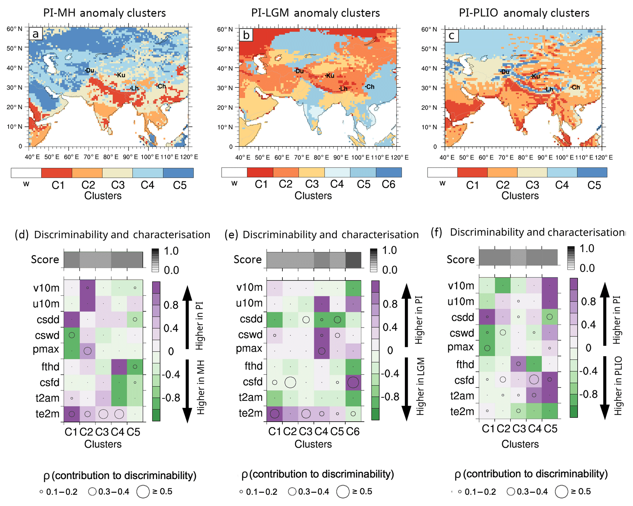
Figure 5The multivariate anomaly maps for time slice comparisons PI–MH (a), PI–LGM (b) and PI–PLIO (c) show the geographical coverage of clusters C1–Ci in the South Asia, which describe the spatial extent of regions characterised by similar modes of change. The corresponding modes of change (d, e, f) for each cluster are expressed as relative changes in each of the nine investigated variables (Table 1): 2 m air temperature (te2 m), 2 m air temperature amplitude (t2am), consecutive freezing days (csfd), freeze–thaw days (fthd), maximum precipitation (pmax), consecutive wet days (cswd), consecutive dry days (csdd), zonal near-surface wind speeds (u10) and meridional near-surface wind speeds (v10). The score (d, e, f) expresses the goodness of discriminability between palaeoclimate pairs PI–MH (d), PI–LGM (e) and PI–PLIO (f) in each of the anomaly clusters. The size of the circles corresponds to the relative contribution of each of the nine climatic attribute variables to the measured discriminability in each anomaly cluster for all three time slice comparisons.
LGM-C1 mostly covers the northernmost parts of the region and the Himalayan orogen (Fig. 5b). The changes associated with it are decreases in 2 m air temperature and increases in 2 m air temperature amplitude and consecutive dry days (Fig. 5e). The modes of change described by LGM-C2 and LGM-C3 govern large parts of the region, including the Arabian Peninsula, Iran, central Asia, the Tibetan Plateau and Tarim basin, Mongolia and parts of China. These regions experience relatively small decreases in temperature. Central India and eastern southeast Asia (LGM-C4) are associated with decreases in consecutive wet days, maximum precipitation and zonal wind speeds, and increases in consecutive dry days. Parts of Kazakhstan, southern Russia, China, southeast Asia and northern India are assigned to LGM-C5, which is characterised by increases in consecutive dry days.
The region covered by PLIO-C1 includes northern India along the Himalayan orogen (Fig. 5c) and experiences decreases in consecutive dry days, and increases in consecutive wet days and maximum precipitation (Fig. 5f). PLIO-C2 covers most of the study region and is associated with relatively little change in all climatic attributes except meridional wind speeds. Central Asia is mostly assigned to PLIO-C3 and experiences an increase in 2 m air temperature and decrease in freeze–thaw days. The north of the study region (PLIO-C4) is characterised by decreases in 2 m air temperature amplitude and consecutive freezing days, and increases in 2 m air temperature and freeze–thaw days. Finally, PLIO-C5 mostly covers the high-altitude locations of the South Asia region that are close to steep topographic gradients, including the Himalayan orogen. This cluster is associated with decreases in wind speeds, consecutive freezing days, consecutive wet days and 2 m air temperature, and with increases in consecutive dry days and 2 m air temperature.
3.3.2 Discriminability
The significance of the climate attributes in explaining the discriminability the South Asia clusters (Fig. 5d, e, f) is more variable than in Europe. While changes in 2 m air temperature are important in most of the MH and LGM results, there is no clear dominant factor for PLIO clusters. In the LGM, the discriminability in the high-altitude/high-latitude cluster (LGM-C1) is mostly explained by decreases in 2 m air temperature (30 %–40 %), mild increases in consecutive freezing days (20 %–30 %) and mild decreases in consecutive wet days (10 %–20 %). LGM-C4 has the second highest discrimination score, and the discrimination in this cluster is explained by decreases in consecutive dry days (10 %–20 %) and increases in consecutive wet days (10 %–20 %), maximum precipitation (30 %–40 %) and 2 m air temperature (20 %–30 %). For PLIO, the type of climate change governing the largest cluster (PLIO-C2) causes discriminability that is primarily explained by mild decreases in consecutive freezing days (20 %–30 %) and mild increases in consecutive wet days (20 %–30 %) and 2 m air temperature amplitude (10 %–20 %). Discriminability in the cluster occupying the region south of the Himalayan orogen (PLIO-C1) is explained by decreases in consecutive dry days (10 %–20 %) and 2 m air temperature (10 %–20 %), and increases in consecutive wet days (10 %–20 %), maximum precipitation (30 %–40 %) and consecutive freezing days (10 %–20 %). Cluster PLIO-C5 is associated with a discriminability best explained by increases in consecutive dry days (30 %–40 %) and decreases in maximum precipitation (10 %–20 %) and consecutive freezing days (20 %–30 %).
This section describes method-related features and problems, and highlights commonly occurring patterns of change, provides possible explanations for those and discusses these changes in the context of erosional processes.
4.1 The role of large-scale features
For many of the LGM and some of the PLIO results, changes in 2 m air temperature and/or consecutive freezing days significantly contribute to the discriminability in clusters covering midlatitudes. LGM-C1–LGM-C3 in coastal and high-altitude west Patagonia (South America), LGM-C1 and PLIO-C4 in the South Asia region are examples of this. Many of these high-latitude clusters are also characterised by large changes in 2 m air temperature and 2 m air temperature amplitude in the LGM and PLIO results. The preferential cooling in higher latitudes during the LGM and enhanced meridional temperature gradient (e.g. Otto-Bliesner et al., 2006; Bracannot et al., 2007; Mutz et al., 2018) can be expected to result in more pronounced seasonality and thus higher variation in near-surface temperature amplitude. Inversely, the accentuated warming in higher latitudes during the (Late) Pliocene (e.g. Salzman et al., 2011; Ballantyne et al., 2010; Mutz et al., 2018) would result in the opposite. These previously studied large-scale features explain much of the characterisation of high-latitude clusters and the significant contribution of changes in temperature-related variables to regional discriminability. Associated changes in temperature variables can have decisive impacts on physical weathering due to changes in glacial and periglacial processes (see below), as well as to biotic weathering by influencing vegetation cover.
4.2 The role of glaciers and periglacial processes
Changes in temperature in high-altitude regions can impact physical weathering through glacial erosion (e.g. Egholm et al., 2009; Herman et al., 2013) and periglacial processes (e.g. Hales and Roering, 2007; Andersen et al., 2015; Marshall et al., 2015). In southernmost South America, northern Europe and southern Alaska (see the Supplement), the high discriminability and modes of change on the multivariate anomaly maps for the LGM are primarily controlled by the glaciers covering most of the region. Furthermore, many modes of change in the study regions involve consecutive freezing days and freeze–thaw days. Changes from ice-free to ice-covered conditions, such as in LGM-C1–LGM-C3 in coastal and high-altitude west Patagonia (South America) and LGM-C1–LGM-C4 in different terrains of Europe, are associated with increases in consecutive freezing days and decreases in freeze–thaw days. The opposite is the case for some modes of changes in the PLIO. For example, PLIO-C6 in high-altitude Patagonia (South America) is associated with changes from ice-covered to ice-free conditions, as well as with an increase in consecutive freezing days. It may therefore shift from glacier to frost-cracking-dominated erosional processes. These modes of change in the PLIO mark a possible transition from glacier-governed processes to periglacial processes and thus increased frost cracking as the Earth's surface spends more time in the frost-cracking window (e.g. Matsuoka, 2001; Schaller et al., 2002; Andersen et al., 2015; Marshall et al., 2015), whereas many LGM modes of change suggest the opposite. Finally, glacial preconditioning of a landscape can modulate the effect of precipitation on landsliding (Moon et al., 2011).
4.3 The role of precipitation characteristics
Areas that have been covered by glaciers during the LGM and experienced a post-LGM increase in maximum precipitation or consecutive wet days may be particularly prone to precipitation-triggered landslides. This is the case, for example, in the regions covered by LGM-C2 and LGM-C3 clusters in high-altitude Patagonia and LGM-C11–LGM-C3 in northern Europe. More generally, changes in storminess affect erosion through river incision and sediment transport (e.g. Whipple and Tucker, 1999; Hobley et al., 2010). Maximum precipitation and consecutive wet days are measures of storm intensity and duration, respectively, which are primary controls for runoff and relevant for erosion. In most cases, such as the results for the South Asia region in the LGM and PLIO, the co-variability of consecutive wet days, maximum precipitation and consecutive dry days is intuitive: changes in consecutive wet days and maximum precipitation coincide with changes in consecutive dry days in the opposite direction. Even though palaeovegetation is considered in the setup of the GCM simulations (Mutz et al., 2018), the modulating effect of vegetation on the impact of changes in the precipitation attribute variables on erosion (e.g. Gyssels et al., 2005) cannot be taken into account here, and thus the reader is advised to do so in their evaluation of the effect of these changes on Earth surface processes. Note also that vegetation modifies river discharge by changing evapotranspiration and infiltration, and modifies hillslope erosion by changing root characteristics (e.g. Schmid et al., 2018). In absence of significant vegetation changes, areas such as Bhutan, Nepal, Bangladesh and parts of northern India (MH-C1 and PLIO-C1), which experience strong increases in consecutive wet days and maximum precipitation in the MH and PLIO, are likely to have experienced an increase in such precipitation-induced erosion at these times.
4.4 The role of winds
Changes in wind speed components affect aeolian erosion, transport and deposition, as well as mean raindrop trajectories, which should also be taken into consideration in the assessment of local precipitation-induced erosion (de Lima et al., 1992). The results of this study reveal that changes in near-surface meridional and zonal wind speeds contribute little to the discriminability between climates even in regions that experience wind direction changes due to a different ice cover in Europe (e.g. Siegert and Dowdeswell, 2004), which are reproduced well by the model. Wind speeds only show a significant contribution to discriminability (20 %–30 %) in the subtropical latitudes of South America due to slower meridional winds in the LGM in the region. The distinctiveness in the character of atmospheric dust transport during the LGM (e.g. Andersen et al., 1998), and thus aeolian erosion may be attributed more to system response and changes in vegetation, which cannot be taken into account in this study, than to a distinctiveness of LGM wind speeds.
4.5 Comments on methodical implications
PLIO and LGM clusters are more stable than MH clusters on the multivariate anomaly maps. This stability can be attributed to the relatively large magnitude of climate change in PLIO and LGM time slices. Lower variance of MH anomalies make element attribution to anomaly clusters in the MH more sensitive to randomisation and re-categorisation procedures (Sect. 2.2). Consequently, the nature of MH patterns can be seen as the result of climate change of lower magnitude and less distinctiveness. The most important limitation is the poor representation of precipitation amount in areas of high topography and rainfall (Meehl et al., 2007 and comparisons with ERA-Interim and station-based observations not presented here). However, the threshold for what constitutes a “wet day” or “dry day” is relatively low (Zolina et al., 2010; Zhang et al., 2011; Zin and Jemain, 2010), so that the typical overestimation of total precipitation amount by ECHAM5 in such regions has little or no effect on the attribute variables “consecutive wet days” and “consecutive dry days”, particularly when analysed in comparison to another simulation at a different time (as was done here), which helps reduce any systematic model bias towards high precipitation rates. Comparisons of the palaeoclimate simulations with local, terrestrial proxy-based reconstructions in South America and South Asia (Li et al., 2017; Mutz et al., 2018) show an agreement of 54 %–59 % in the MH, and 65 %–100 % in the LGM. Erosion-relevant processes that take place on small spatial or short temporal scales, such as intra-storm variations and rainfall characteristics (e.g. Ran et al., 2012), cannot be quantified in this study due to limited model resolution, output frequency and accuracy of such estimates on that scale. The consideration of non-climatic factors, such as local topography, slope and vegetation, is beyond the scope of this study, and the reader is advised to take these into consideration in their assessment of the effect of documented climate change on Earth surface processes. Lastly, since the parameterisation in ECHAM5's land surface scheme creates deficiencies in the representation of the local hydrology and partitioning of precipitation (e.g. Weiland et al., 2011), variables such as runoff are excluded in this study. Routing GCM output through more sophisticated hydrological models or nesting regional climate models in the GCMs would allow more merited exploration of the regional hydrology.
In this study, we quantified the differences between pre-industrial and Late Cenozoic palaeoclimates with regard to variables relevant to Earth surface processes, explained these quantified differences and identified dominant patterns and modes of palaeoclimate change. The key findings of this study are as follows:
-
Last Glacial Maximum and Mid-Pliocene climate change is more distinct and more easily quantified than climate change of the Mid-Holocene. This is reflected in the stability of geographical regions (clusters) showing the extent of regions governed by distinct modes of climate change.
-
Changes in ice cover result in distinct signatures of climate change. This is reflected by (1) the creation of clusters geographically associated with ice cover changes, (2) the persistence of these clusters when the assigned number of clusters (k) is varied in the procedure and (3) ice cover changes in South America leading to the best discriminability overall.
-
In Europe, changes in 2 m air temperature explain most of the discriminability between pre-industrial and all three palaeoclimates (Mid-Holocene, Last Glacial Maximum and Mid-Pliocene). Changes in consecutive freezing days and consecutive wet days are also significant contributors to climate discriminability in Last Glacial Maximum and Mid-Pliocene results, respectively. Consequently, these factors lend the Late Cenozoic palaeoclimates their unique signature and should be central in assessments of changes in Earth surface processes.
-
Increases in freeze–thaw days and temperature often coincide with decreases in consecutive freezing days, and vice versa. Regions governed by these modes of changes, such as western Patagonia during the Last Glacial Maximum, are prone to changes in erosional process domain from peri-glacial to glacial, or vice versa.
-
Increases in consecutive wet days and maximum precipitation often coincide with decreases in consecutive dry days. Regions governed by these modes of change, such as locations south of the Himalayan orogen in the Mid-Pliocene, can be expected to be particularly prone to changes in erosion induced by precipitation and storm characteristics.
We note that the methods presented in this study may also be applied to simulations of modern and future climates. Furthermore, the procedure can easily be modified to detect and explain spatiotemporal changes in climate attributes associated with different processes, since the link between climate and the impacted system is established solely on the basis of variable selection. For example, the procedure may be used for the investigation of spatiotemporal changes of climate attributes that are related to specific human adaptation strategies in the past or future. Such method transfer is merited if (1) the underlying statistical assumptions are still satisfied and (2) the chosen variables adequately represent the relationship between climate and the investigated processes. The procedure may also be applied more broadly to any problem that requires the detection of regions (in either geographical or any nth dimensional variable space) associated with specific modes of change in data, and the subsequent quantification and explanation of changes occurring within identified regions.
All data files used in the presentation of results, as well as the model simulation results in this study based on Mutz et al. (2018), are freely available through the data download section of our work group wiki (https://esdynamics.geo.uni-tuebingen.de/wiki/index.php/data-download, last access: 19 July 2019) as a set of data products tailored to the needs of different geoscientific communities.
The supplement related to this article is available online at: https://doi.org/10.5194/esurf-7-663-2019-supplement.
SGM's contribution includes experiment design and implementation, interpretation of results and writing the manuscript. TAE contributed to experiment design, interpretation of results and manuscript editing.
The authors declare that they have no conflict of interest.
European Research Council (ERC) consolidator grant number 615703 provided support for this study. Additional support is acknowledged from the German science foundation (DFG) project number 365266215. We also thank the reviewers (including Andrew Wickert) and editor (Simon Mudd) for their constructive comments and suggestions, which helped us improve the manuscript.
This research has been supported by the European Research Council (grant no. 615703) and the German science foundation (DFG; project no. 365266215).
This open-access publication was funded
by the University of Tübingen.
This paper was edited by Simon Mudd and reviewed by Andrew Wickert and one anonymous referee.
Abe-Ouchi, A., Saito, F., Kageyama, M., Braconnot, P., Harrison, S. P., Lambeck, K., Otto-Bliesner, B. L., Peltier, W. R., Tarasov, L., Peterschmitt, J.-Y., and Takahashi, K.: Ice-sheet configuration in the CMIP5/PMIP3 Last Glacial Maximum experiments, Geosci. Model Dev., 8, 3621–3637, https://doi.org/10.5194/gmd-8-3621-2015, 2015.
Andersen, J. L., Egholm, D. L., Knudsen, M. F., Jansen, J. D., and Nielsen, S. B.: The periglacial engine of mountain erosion – Part 1: Rates of frost cracking and frost creep, Earth Surf. Dynam., 3, 447–462, https://doi.org/10.5194/esurf-3-447-2015, 2015.
Andersen, K. K., Armengaud, A., and Genthon, C.: Atmospheric dust under glacial and interglacial conditions, Geophys. Res. Lett., 25, 2281–2284, 1998.
Bahrenberg, G., Giese, E., and Nipper, J.: Multivariate Statistik. Statistische Methoden in der Geographie 2, Teubner, Stuttgart, Germany, 1992.
Ballantyne, A. P., Greenwood, D. R., Sinninghe Damste, J. S., Csank, A. Z., Eberle, J. J., and Rybczynski, N.: Significantly warmer Arctic surface temperatures during the Pliocene indicated by multiple independent proxies, Geology, 38, 603–606, 2010.
Bigelow, N. H., Brubaker, L. B., Edwards, M. E., Harrison, S. P., Prentice, I. C., Anderson, P. M., Andreev, A. A., Bartlein, P. J., Christensen, T. R., Cramer, W., Kaplan, J. O., Lozhkin, A. V., Matveyeva, N. V., Murray, D. V., McGuire, A. D., Razzhivin, V. Y., Ritchie, J. C., Smith, B., Walker, D. A., Gajewski, K., Wolf, V., Holmqvist, B. H., Igarashi, Y., Kremenetskii, K., Paus, A., Pisaric, M. F. J., and Vokova, V. S.: Climate change and Arctic ecosystems I. Vegetation changes north of 55∘ N between the last glacial maximum, mid-Holocene and present, J. Geophys. Res.-Atmos., 108, 8170, https://doi.org/10.1029/2002JD002558, 2003.
Bookhagen, B., Thiede, R. C., and Strecker, M. R.: Late Quarternary intensified monsoon phases control landscape evolution in the northwest Himalaya, Geology, 33, 149–152, https://doi.org/10.1130/G20982.1, 2005.
Braconnot, P., Otto-Bliesner, B., Harrison, S., Joussaume, S., Peterchmitt, J.-Y., Abe-Ouchi, A., Crucifix, M., Driesschaert, E., Fichefet, Th., Hewitt, C. D., Kageyama, M., Kitoh, A., Laîné, A., Loutre, M.-F., Marti, O., Merkel, U., Ramstein, G., Valdes, P., Weber, S. L., Yu, Y., and Zhao, Y.: Results of PMIP2 coupled simulations of the Mid-Holocene and Last Glacial Maximum – Part 1: experiments and large-scale features, Clim. Past, 3, 261–277, https://doi.org/10.5194/cp-3-261-2007, 2007.
Braconnot, P., Harrison, S. P., Kageyama, M., Bartlein, P. J., Masson-Delmotte, V., Abe-Ouchi, A., Otto-Bliesner, B., and Zhao, Y.: Evaluation of climate models using palaeoclimatic data, Nat. Clim. Change, 2, 417–424, 2012.
CLIMAP Project Members: Seasonal Reconstruction of the Earth's Surface at the Last Glacial Maximum, Map and Chart Series, vol. 36, Geological Society of America, Boulder, Colorado, USA, 18 pp., 1981.
Deal, E., Braun, J., and Botter, G.: Understanding the Role of Rainfall Hydrology in Determining Fluvial Erosion Efficiency, J. Geophys. Res.-Earth, 123, 744–778, https://doi.org/10.1002/2017JF004393, 2018.
de Lima, J. L. M. P., van Dijk, P. M., and Spaan, W. P.: Splash-saltation transport under wind-driven rain, Soil Technol., 5, 151–166, https://doi.org/10.1016/0933-3630(92)90016-T, 1992.
Dowsett, H. J., Robinson, M., Haywood, A., Salzmann, U., Hill, D., Sohl, L., Chandler, M., Williams, M., Foley, K., and Stoll, D.: The PRISM3D paleoenvironmental reconstruction, Stratigraphy, 7, 123–139, 2010.
Egholm, D. L., Nielsen, S. B., Pedersen, V. K., and Lesemann, J.: Glacial efects limiting moutain height, Nature, 460, 884–887, 2009.
Ehlers, T. A. and Poulsen, C. J.: Influence of Andean uplift on climate and paleoaltimetry estimates, Earth Planet. Sc. Lett., 281, 238–248, 2009.
Gong, X., Knorr, G., Lohmann, G., and Zhang, X.: Dependence of abrupt Atlantic meridional ocean circulation changes on climate background states, Geophys. Res. Lett., 40, 3698–3704, https://doi.org/10.1002/grl.50701, 2013.
Gyssels, G., Poesen, J., Bochet, E., and Li, Y.: Impact of plant roots on the resistance of soils to erosion by water: a review, Prog. Phys. Geog., 29, 189–217, https://doi.org/10.1191/0309133305pp443ra, 2005.
Hales, T.-C. and Roering, J. J.: Climatic controls on frost cracking and implications for the evolution of bedrock landscapes, J. Geophys. Res., 112, F02033, https://doi.org/10.1029/2006JF000616, 2007.
Harrison, S. P., Yu, G., Takahara, H., and Prentice, I. C.: Palaeovegetation – Diversity of temperate plants in east Asia, Nature, 413, 129–130, 2001.
Haywood, A. M., Dowsett, H. J., Otto-Bliesner, B., Chandler, M. A., Dolan, A. M., Hill, D. J., Lunt, D. J., Robinson, M. M., Rosenbloom, N., Salzmann, U., and Sohl, L. E.: Pliocene Model Intercomparison Project (PlioMIP): experimental design and boundary conditions (Experiment 1), Geosci. Model Dev., 3, 227–242, https://doi.org/10.5194/gmd-3-227-2010, 2010.
Haywood, A. M., Hill, D. J., Dolan, A. M., Otto-Bliesner, B. L., Bragg, F., Chan, W.-L., Chandler, M. A., Contoux, C., Dowsett, H. J., Jost, A., Kamae, Y., Lohmann, G., Lunt, D. J., Abe-Ouchi, A., Pickering, S. J., Ramstein, G., Rosenbloom, N. A., Salzmann, U., Sohl, L., Stepanek, C., Ueda, H., Yan, Q., and Zhang, Z.: Large-scale features of Pliocene climate: results from the Pliocene Model Intercomparison Project, Clim. Past, 9, 191–209, https://doi.org/10.5194/cp-9-191-2013, 2013.
Haywood, A. M., Dowsett, H. J., Dolan, A. M., Rowley, D., Abe-Ouchi, A., Otto-Bliesner, B., Chandler, M. A., Hunter, S. J., Lunt, D. J., Pound, M., and Salzmann, U.: The Pliocene Model Intercomparison Project (PlioMIP) Phase 2: scientific objectives and experimental design, Clim. Past, 12, 663–675, https://doi.org/10.5194/cp-12-663-2016, 2016.
Herman, F., Seward, D., Valla, P. G., Carter, A., Kohn, B., Willet, S. D., and Ehlers, T. A.: Worldwide acceletation of mountain erosion under a cooling climate, Nature, 504, 423–426, 2013.
Hobley, D. E., Sinclair, H. D., and Cowie, P. A.: Processes, rates, and time scales of fluvial response in an ancient postglacial landscape of the northwest Indian Himalaya, Geol. Soc. Am. Bull., 122, 1569–1584, 2010.
Insel, N., Ehlers, T. A., Schaller, M., Barnes, J. B., Tawacoli, S., and Poulsen, C. J.: Spatial and Temporal Variability in Denudation across the Bolivian Andes from Multiple Geochronometers, Geomorphology, 122, 65–77, https://doi.org/10.1016/j.geomorph.2010.05.014, 2010.
Jeffery, M. L., Ehlers, T. A., Yanites, B. J., and Poulsen, C. J.: Quantifying the role of paleoclimate and Andean Plateau uplift on river incision: PALEOCLIMATE ROLE IN RIVER INCISION, J. Geophys. Res.-Earth, 118, 852–871, https://doi.org/10.1002/jgrf.20055, 2013.
Jungclaus, J. H., Lorenz, S. J., Timmreck, C., Reick, C. H., Brovkin, V., Six, K., Segschneider, J., Giorgetta, M. A., Crowley, T. J., Pongratz, J., Krivova, N. A., Vieira, L. E., Solanki, S. K., Klocke, D., Botzet, M., Esch, M., Gayler, V., Haak, H., Raddatz, T. J., Roeckner, E., Schnur, R., Widmann, H., Claussen, M., Stevens, B., and Marotzke, J.: Climate and carbon-cycle variability over the last millennium, Clim. Past, 6, 723–737, https://doi.org/10.5194/cp-6-723-2010, 2010.
Kageyama, M., Albani, S., Braconnot, P., Harrison, S. P., Hopcroft, P. O., Ivanovic, R. F., Lambert, F., Marti, O., Peltier, W. R., Peterschmitt, J.-Y., Roche, D. M., Tarasov, L., Zhang, X., Brady, E. C., Haywood, A. M., LeGrande, A. N., Lunt, D. J., Mahowald, N. M., Mikolajewicz, U., Nisancioglu, K. H., Otto-Bliesner, B. L., Renssen, H., Tomas, R. A., Zhang, Q., Abe-Ouchi, A., Bartlein, P. J., Cao, J., Li, Q., Lohmann, G., Ohgaito, R., Shi, X., Volodin, E., Yoshida, K., Zhang, X., and Zheng, W.: The PMIP4 contribution to CMIP6 – Part 4: Scientific objectives and experimental design of the PMIP4-CMIP6 Last Glacial Maximum experiments and PMIP4 sensitivity experiments, Geosci. Model Dev., 10, 4035–4055, https://doi.org/10.5194/gmd-10-4035-2017, 2017.
Kageyama, M., Braconnot, P., Harrison, S. P., Haywood, A. M., Jungclaus, J. H., Otto-Bliesner, B. L., Peterschmitt, J.-Y., Abe-Ouchi, A., Albani, S., Bartlein, P. J., Brierley, C., Crucifix, M., Dolan, A., Fernandez-Donado, L., Fischer, H., Hopcroft, P. O., Ivanovic, R. F., Lambert, F., Lunt, D. J., Mahowald, N. M., Peltier, W. R., Phipps, S. J., Roche, D. M., Schmidt, G. A., Tarasov, L., Valdes, P. J., Zhang, Q., and Zhou, T.: The PMIP4 contribution to CMIP6 – Part 1: Overview and over-arching analysis plan, Geosci. Model Dev., 11, 1033–1057, https://doi.org/10.5194/gmd-11-1033-2018, 2018.
Knorr, G., Butzin, M., Micheels, A., and Lohmann, G.: A Warm Miocene Climate at Low Atmospheric CO2 levels, Geophys. Res. Lett., 38, L20701, https://doi.org/10.1029/2011GL048873, 2011.
Kutzbach, J. E., Prell, W. L., and Ruddiman, W.F .: Sensitivity of Eurasian Climate to Surface Uplift of the Tibetan Plateau, J. Geol., 101, 177–190, 1993.
Li, J., Ehlers, T. A., Werner, M., Mutz, S. G., Steger, C., and Paeth, H.: Late quarternary climate, precipitation δ18O, and Indian monsoon variations over the Tibetan Plateau, Earth Planet. Sc. Lett., 457, 412–422, 2017.
Lohmann, G., Pfeiffer, M., Laepple, T., Leduc, G., and Kim, J.-H.: A model–data comparison of the Holocene global sea surface temperature evolution, Clim. Past, 9, 1807–1839, https://doi.org/10.5194/cp-9-1807-2013, 2013.
Maroon, E. A., Frierson, D. M. W., and Battisti, D. S.: The tropical precipitation response to Andes topography and ocean heat fluxes in an aquaplanet model, J. Climate, 28, 381–398, https://doi.org/10.1175/JCLI-D-14-00188.1, 2015.
Maroon, E. A., Frierson, D. M. W., Kang, S. M., and Scheff, J.: The precipitation response to an idealized subtropical continent, J. Climate, 29, 4543–4564, https://doi.org/10.1175/JCLI-D-15-0616.1, 2016.
Marshall, J. A., Roering, J. J., Bartlein, P. J., Gavin, D. G., Granger, D. E., Rempel, A. W., Praskievicz, S. J., and Hales, T. C.: Frost for the trees: Did climate increase erosion in unglaciated landscapes during the late Pleistocene?, Sci. Adv., 1, 1–10, 2015.
Matsuoka, N.: Solifluction rates, processes and landforms: A global review, Earth-Sci. Rev., 55, 107–134, 2001.
Meehl, G. A., Covey, C., Delworth, T., Latif, M., McAvaney, B., Mitchell, J. F. B., Stouffer, R. J., and Taylor, K. E.: The WCRP CMIP3 multi-model dataset: A new era in climate change research, B. Am. Meterol. Soc., 88, 1383–1394, 2007.
Montgomery, D. R., Balco, G., and Willett, S.D.: Climate, tectonics, and the morphology of the Andes, Geology, 29, 579–582, 2001.
Moon, S., Chamberlain, C. P., Blisniuk, K., Levine, N., Rood, D. H., and Hilley, G. E.: Climatic control of denudation in the deglaciated landscape of the Washington Cascades, Nat. Geosci., 4, 469–473, 2011.
Mutz, S. G., Ehlers, T. A., Li, J., Steger, C., Peath, H., Werner, M., and Poulsen, C. J.: Precipitation δ18O over the South Asia Orogen from ECHAM5-wiso Simulation: Statistical Analysis of Temperature, Topography and Precipitation, J. Geophys. Res.-Atmos., 121, 9278–9300, https://doi.org/10.1002/2016JD024856, 2016.
Mutz, S. G., Ehlers, T. A., Werner, M., Lohmann, G., Stepanek, C., and Li, J.: Estimates of late Cenozoic climate change relevant to Earth surface processes in tectonically active orogens, Earth Surf. Dynam., 6, 271–301, https://doi.org/10.5194/esurf-6-271-2018, 2018.
Otto-Bliesner, B. L., Brady, C. B., Clauzet, G., Tomas, R., Levis, S., and Kothavala, Z.: Last Glacial Maximum and Holocene Climate in CCSM3, J. Climate, 19, 2526–2544, 2006.
Otto-Bliesner, B. L., Braconnot, P., Harrison, S. P., Lunt, D. J., Abe-Ouchi, A., Albani, S., Bartlein, P. J., Capron, E., Carlson, A. E., Dutton, A., Fischer, H., Goelzer, H., Govin, A., Haywood, A., Joos, F., LeGrande, A. N., Lipscomb, W. H., Lohmann, G., Mahowald, N., Nehrbass-Ahles, C., Pausata, F. S. R., Peterschmitt, J.-Y., Phipps, S. J., Renssen, H., and Zhang, Q.: The PMIP4 contribution to CMIP6 – Part 2: Two interglacials, scientific objective and experimental design for Holocene and Last Interglacial simulations, Geosci. Model Dev., 10, 3979–4003, https://doi.org/10.5194/gmd-10-3979-2017, 2017.
Paeth, H.: Key Factors in African Climate Change Evaluated by a Regional Climate Model, Erdkunde, 58, 290–315, 2004.
Pfeiffer, M. and Lohmann, G.: Greenland Ice Sheet influence on Last Interglacial climate: global sensitivity studies performed with an atmosphere–ocean general circulation model, Clim. Past, 12, 1313–1338, https://doi.org/10.5194/cp-12-1313-2016, 2016.
Pickett, E. J., Harrison, S. P., Flenley, J., Grindrod, J., Haberle, S., Hassell, C., Kenyon, C., MacPhail, M., Martin, H., Martin, A. H., McKenzie, M., Newsome, J. C., Penny, D., Powell, J., Raine, J. I., Southern, W., Stevenson, J., Sutra, J.-P., Thomas, I., van der Kaars, S., and Ward, J.: Pollen-based reconstructions of biome distributions for Australia, South-East Asia and the Pacific (SEAPAC region) at 0, 6000 and 18,000 14C years B.P., J. Biogeogr., 31, 1381–1444, https://doi.org/10.1111/j.1365-2699.2004.01001.x, 2004.
Prentice, I. C., Jolly, D., and BIOME 6000 Participants: Mid-Holocene and glacial-maximum vegetation geography of the northern continents and Africa, J. Biogeogr., 27, 507–519, 2000.
Ran, Q., Su, D., Li, P., and He, Z.: Experimental study of the impact of rainfall characteristics on runoff generation and soil erosion, J. Hydrol., 424–425, 99–111, 2012.
Salzmann, U., Williams, M., Haywood, A. M., Johnson, A. L. A., Kender, S., and Zalasiewicz, J.: Climate and environment of a Pliocene warm world, Palaeogeogr. Palaeocl., 309, 1–8, https://doi.org/10.1016/j.palaeo.2011.05.044, 2011.
Sarnthein, M., Gersonde, R., Niebler, S., Pflaumann, U., Spielhagen, R., Thiede, J., Wefer, G., and Weinelt, M.: Overview of Glacial Atlantic Ocean Mapping (GLAMAP 2000), Paleoceanography, 18, 1030, https://doi.org/10.1029/2002PA000769, 2003.
Schaller, M., von Blanckenburg, F., Veldkamp, A., Tebbens, L. A., Hovius, N., and Kubik, P. W.: A 30 000 yr record of erosion rates from cosmogenic 10 Be in Middle European river terraces, Earth Planet. Sc. Lett., 204, 307–320, 2002.
Schmid, M., Ehlers, T. A., Werner, C., Hickler, T., and Fuentes-Espoz, J.-P.: Effect of changing vegetation and precipitation on denudation – Part 2: Predicted landscape response to transient climate and vegetation cover over millennial to million-year timescales, Earth Surf. Dynam., 6, 859–881, https://doi.org/10.5194/esurf-6-859-2018, 2018.
Siegert, M. J. and Dowdeswell, J. A.: Numerical reconstruction of the Eurasian Ice Sheet and climate during the Late Weichselian, Quaternary Sci. Rev., 23, 1273–1283, 2004.
Sohl, L. E., Chandler, M. A., Schmunk, R. B., Mankoff, K., Jonas, J. A., Foley, K. M., and Dowsett, H. J.: PRISM3/GISS topographic reconstruction, U.S. Geological Survey Data Series, 419, 6 pp., available at: https://pubs.usgs.gov/ds/419/DS419.pdf (last access: 19 July 2019), 2009.
Starke, J., Ehlers, T. A., and Schaller, M.: Tectonic and Climatic Controls on the Spatial Distribution of Denudation Rates in Northern Chile (18∘ S–23∘ S) Determined From Cosmogenic Nuclides, J. Geophys. Res.-Earth, 122, 1949–1971, https://doi.org/10.1002/2016JF004153, 2017.
Stepanek, C. and Lohmann, G.: Modelling mid-Pliocene climate with COSMOS, Geosci. Model Dev., 5, 1221–1243, https://doi.org/10.5194/gmd-5-1221-2012, 2012.
Stock, G. M., Frankel K. L., Ehlers, T. A., Schaller, M., Briggs, S. M., and Finkel R. C.: Spatial and temporal variations in denudation of the Wasatch Mountains, Utah, USA, Lithosphere GSA, vol. 1, 34–40, https://doi.org/10.1130/L15.1, 2009.
Takahashi, K. and Battisti, D.: Processes controlling the mean tropical pacific precipitation pattern. Part I: The Andes and the eastern Pacific ITCZ, J. Climate, 20, 3434–3451, 2007.
Wei, W. and Lohmann, G.: Simulated Atlantic Multidecadal Oscillation during the Holocene, J. Climate, 25, 6989–7002, https://doi.org/10.1175/JCLI-D-11-00667.1, 2012.
Weiland, F. C. S., van Beek, L. P. H., Kwadjik, J. C. J., and Bierkens, M. F. P.: On the Suitability of GCM Runoff Fields for River Discharge Modelling: A Case Study Using Model Output from HadGEM2 and ECHAM5, J. Hydrometeorol., 13, 140–154, 2011.
Whipple, K. X.: The influence of climate on the tectonic evolution of mountain belts, Nat. Geosci., 2, 97–104, https://doi.org/10.1038/ngeo413, 2009.
Whipple, K. X. and Tucker, G. E.: Dynamics of the stream-power river incision model: Implications for height limits of mountain ranges, landscape response timescales, and research needs, J. Geophys. Res.-Sol. Ea., 104, 17661–17674, 1999.
Wickert, A. D.: Reconstruction of North American drainage basins and river discharge since the Last Glacial Maximum, Earth Surf. Dynam., 4, 831–869, https://doi.org/10.5194/esurf-4-831-2016, 2016.
Wilks, D. S.: Statistical methods in the atmospheric sciences, 3rd ed., Academic Press, Oxford, UK, 2011.
Willett, S. D., Schlunegger, F., and Picotti, V.: Messinian climate change and erosional destruction of the central European Alps, Geology, 34, 613–616, 2006.
Zhang, Q., Singh, V. P., Li, J., and Chen, X.: Analysis of periods of maximum consecutive wet days in China, J. Geophys. Res., 116, D23106, https://doi.org/10.1029/2011JD016088, 2011.
Zhang, X., Lohmann, G., Knorr, G., and Purcell, C.: Abrupt glacial climate shifts controlled by ice sheet changes, Nature, 512, 290–294, https://doi.org/10.1038/nature13592, 2014.
Zin, W. Z. W. and Jemain, A. A.: Statistical distributions of extreme dry spell in Peninsular Malaysia, Theor. Appl. Climatol., 102, 253–264, 2010.
Zolina, O., Simmer, C., Gulev, S. K., and Kollet, S.: Changing structure of European precipitation: Longer wet periods leading to more abundant rainfall, Geophys. Res. Lett., 37, L06704, https://doi.org/10.1029/2010GL042468, 2010.