the Creative Commons Attribution 4.0 License.
the Creative Commons Attribution 4.0 License.
 | 17 Jan 2019
Short communication: flow as distributed lines within the landscape
Landscape evolution models (LEMs) aim to capture an aggregation of the processes of erosion and deposition within the earth's surface and predict the evolving topography. Over long timescales, i.e. greater than 1 million years, the computational cost is such that numerical resolution is coarse and all small-scale properties of the transport of material cannot be captured. A key aspect, therefore, of such a long timescale LEM is the algorithm chosen to route water down the surface. I explore the consequences of two end-member assumptions of how water flows over the surface of an LEM – either down a single flow direction (SFD) or down multiple flow directions (MFDs) – on model sediment flux and valley spacing. I find that by distributing flow along the edges of the mesh cells, node to node, the resolution dependence of the evolution of an LEM is significantly reduced. Furthermore, the flow paths of water predicted by this node-to-node MFD algorithm are significantly closer to those observed in nature. This reflects the observation that river channels are not necessarily fixed in space, and a distributive flow captures the sub-grid-scale processes that create non-steady flow paths. Likewise, drainage divides are not fixed in time. By comparing results between the distributive transport-limited LEM and the stream power model “Divide And Capture”, which was developed to capture the sub-grid migration of drainage divides, I find that in both cases the approximation for sub-grid-scale processes leads to resolution-independent valley spacing. I would, therefore, suggest that LEMs need to capture processes at a sub-grid-scale to accurately model the earth's surface over long timescales.
- Article
(4070 KB) - Full-text XML
- BibTeX
- EndNote


It is known that resolution impacts landscape evolution models (LEMs) (Schoorl et al., 2000). The resolution dependence of LEMs is caused by how run-off is routed down the model surface. It has been demonstrated that either distributing flow down all slopes (multiple flow direction, MFD) or simply allowing flow to descend down the steepest slope (single flow direction, SFD), gives different outcomes for landscape evolution models (Pelletier, 2004; Schoorl et al., 2000). It has been noted that landscape potentially has a characteristic wavelength for the spacing of valleys (Perron et al., 2008). Therefore, a landscape evolution model should be able to reproduce such regular topographic features independently of the model resolution. For a model of channelized flow, it was, however, found that the routing of run-off led to a resolution dependence in the valley spacing, which could be overcome by the addition of a parameterized flow width that was less than the numerical grid spacing (Perron et al., 2008).
There is a potential problem with parameterizing the flow width to be fixed at a sub grid level. The response time of LEMs to a change in external forcing is strongly dependent on the surface run-off (Armitage et al., 2018). This means that the model response time becomes likewise dependent on the chosen flow width. Ideally, the LEM would be independent of grid resolution without introducing a predefined length scale that impacts the model response.
Water is the primary agent of landscape erosion. There are multiple pathways within the hydrological cycle from evaporation, transpiration, and groundwater flow; however, for many landscapes the river network is the primary route through which water flows downslope. Mean river width varies from 5 km to a few metres (Allen and Pavelsky, 2018). The very wide rivers, greater than 1 km, are, however, outliers within this global data set, with the median of the distribution of mean river width being 124 m, with the upper quartile at 432 m (Fig. 1). In LEMs developed for understanding long-term landscape evolution, the large timescales necessitate large spatial scales, where a single grid cell can be 1 km wide or more (Temme et al., 2017). A spatial resolution of cells larger than a few metres becomes necessary when modelling at the scale of a continent (Salles et al., 2017). This means that flow has a width at a subgrid level.
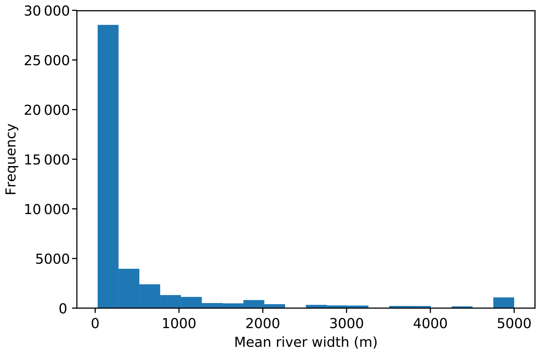
Figure 1Distribution of mean river width taken from the Global River Widths from Landsat (GRWL) Database (Allen and Pavelsky, 2018).
If the width of the flow path for run-off is narrower than can be reasonably modelled, then can the flow paths be treated as lines, from model node to node (Fig. 2), where water collects along these lines? To explore this idea and understand LEM sensitivity to resolution, I wish to explore how a simple LEM evolves under four scenarios (Fig. 2): (1) simple SFD from cell area to cell area, (2) an MFD version of this cell-to-cell algorithm, (3) a node-to-node SFD, and (4) a node-to-node MFD.
In this study I will assume landscape evolution can be effectively simulated with the classic set of diffusive equations described in Smith and Bretherton (1972):
where κ is a linear diffusion coefficient, c is the fluvial diffusion coefficient, qw is the water flux, n is the water flux exponent, and U is uplift. This heuristic concentrative–diffusive equation is capable of generating realistic landscape morphology, with the slope–area relationships commonly observed (Armitage et al., 2018; Simpson and Schlunegger, 2003). Strictly, it assumes that there is always a layer of material to be transported by surface run-off, and as such it can be classed as a transport-limited model. It accounts for both erosion and deposition and is, therefore, appropriate for modelling landscape evolution beyond mountain ranges and into the depositional setting (see models such as DIONISOS; Granjeon and Joseph, 1999). It differs from mixed erosion and deposition models such as Kooi and Beaumont (1994) and Davy and Lague (2009) because those models split the divergence of the sediment flux into two terms: a rate of erosion and a rate of deposition. Here, instead I assume that the sediment flux is a function of water flux and slope.
Equation (1) is solved with a finite-element scheme written using Python and the FEniCS libraries (I will call the code “fLEM”; see the “Code availability” section). The equations are solved on a Delaunay mesh, where the mesh is made up of predominantly equilateral triangles with an opening angle of 60∘. Model boundary conditions are initially of fixed elevation on the sides normal to the x axis and a zero gradient on the sides normal to the y axis. The model aspect ratio is 4 to 1. Uplift is fixed at m yr−1, the linear diffusion coefficient is κ=1 m2 yr−1, the fluvial diffusion coefficient is (m2 yr−1)n−1, and the water flux exponent is n=1.5.
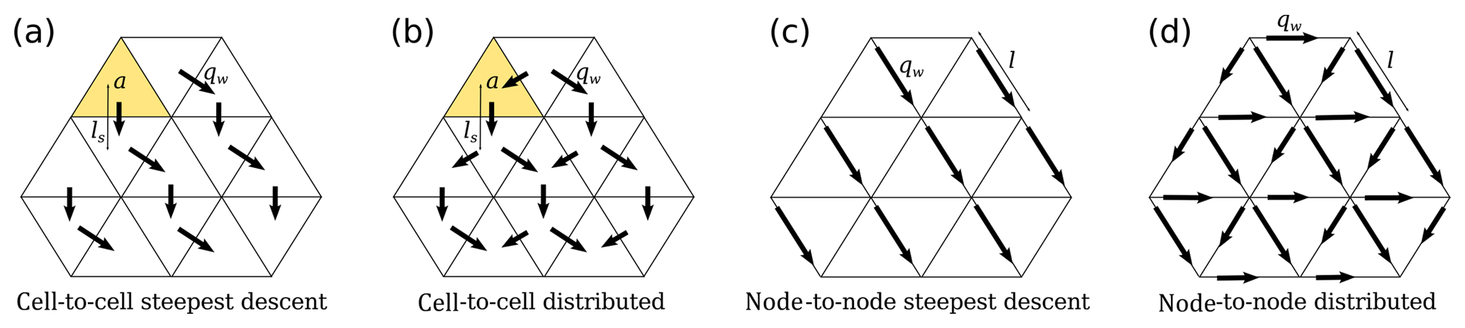
Figure 2Diagram of flow routing from cell to cell and node to node for either a single flow direction (SFD) or a multiple flow direction (MFD) algorithm weighted by the relative gradient.
Water can be routed from cell to cell, where precipitation is collected over the area of each cell, sent downwards, and accumulates. In this cell-to-cell configuration the water flux has units of length squared per unit time and is given by
where α is precipitation rate, a is the cell area, and ls is the length from cell centre to cell centre down the steepest slope (Fig. 2a and b). This gives a water discharge per unit length, which has the advantage of not having to explicitly state the sub-grid width of the flow (Simpson and Schlunegger, 2003). However, implicitly this implies that the flow is over the width of a cell. An alternative is to route water from node to node along cell edges and for it to accumulate. I assume that along the length of each cell edge water can be added to the flow line, assuming that the input is linearly related to the length of the flow line,
where l is the length of the edge that joins the upslope node to the downslope node (Fig. 2c and d). This means that the cell area is ignored and instead water enters the flow path uniformly along its length and accumulates downslope.
Equation (3) makes the assumption that water accumulates as a function of length. Water flux is observed to be related to catchment area: Qw∝A0.8 (Syvitski and Milliman, 2007). The catchment length, l, is then related to area by , where (Armitage et al., 2018). At the lower end of the range, this gives Qw∝l1.12, suggesting that accumulating water as a linear function of flow length is a reasonable simplification. A knock-on effect of this assumption is that the magnitude of the water flux predicted for the node-to-node routing is less than that of the cell-to-cell, as in the latter water is accumulated over cell areas which is naturally larger than the cells' edges.
Both Eqs. (2) and (3) do not attempt to capture the interaction between water flux and river width; rather, these are two methods to approximate run-off within a coarse numerical grid. For both the cell-to-cell and node-to-node methods the flow can then be routed down a SFD or routed down MFDs weighted by the relative gradient, as in, for example, Schoorl et al. (2000). I run the numerical model with a uniform precipitation rate of α=1 m yr−1.
Equation (1) is made dimensionless following Simpson and Schlunegger (2003) using the linear diffusion timescale and the model length in the x direction, L. This means that Eq. (1) can be rewritten as
and
where , , , , , and
At a low model resolution, 512×128 cells, all four methods of flow routing give a similar landscape morphology after 5 Myr of model evolution (Figs. 3 and 4). However, elevations are significantly lower for the cell-to-cell flow routing model as the water flux term is lower for the node-to-node routing algorithm (Figs. 3 and 4). As the resolution is increased to 2048×512 cells, the landscape morphology starts to diverge. For the cell-to-cell SFD algorithm, the landscape shows more small-scale branching, as previously discussed by Braun and Sambridge (1997) (Fig. 3b and c). For the SFD algorithm it can be seen that the high-resolution model has multiple peaks along the ridges (Fig. 3b). This roughness to the topography is removed if the flow is distributed downslope from cell to cell (MFD; Fig. 3d).
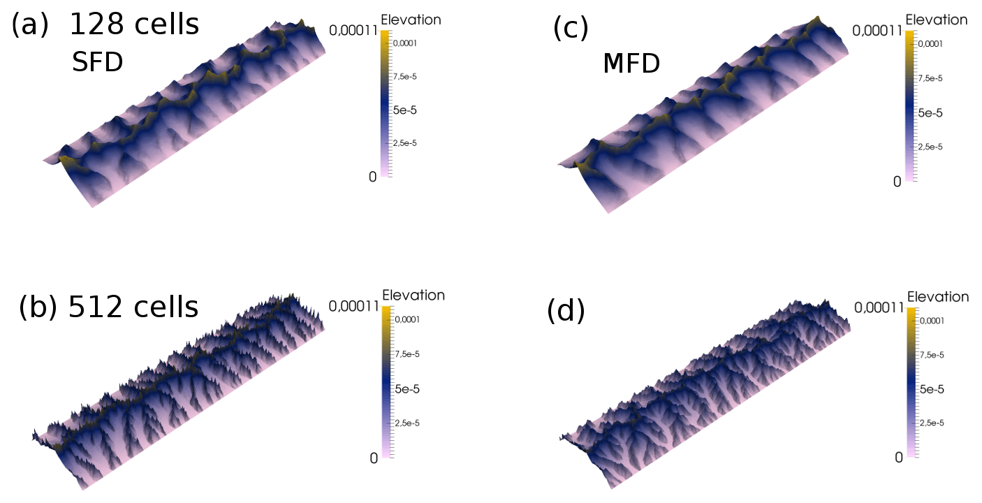
Figure 3Dimensionless elevation from the cell-to-cell flow routing landscape evolution model with different flow routing algorithms at different numerical resolutions after a dimensionless runtime of (5 Myr), with an aspect ratio of 4×1. (a) Cell-to-cell single flow direction (SFD) algorithm with a resolution of 512×128 cells. (b) The same model but with a resolution of 2048×512 cells. Panels (c) and (d): cell-to-cell multiple flow direction (MFD) algorithm.
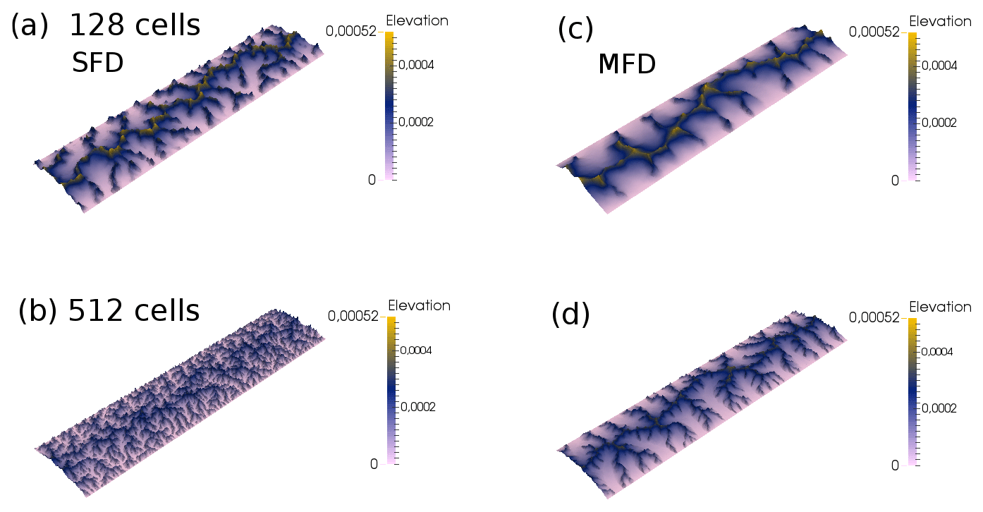
Figure 4Dimensionless elevation from the node-to-node flow routing landscape evolution model with different flow routing algorithms at different numerical resolutions after a dimensionless runtime of (5 Myr), with an aspect ratio of 4×1. (a) Node-to-node single flow direction (SFD) algorithm with a resolution of 512×128 cells. (b) The same model but with a resolution of 2048×512 cells. Panels (c) and (d): node-to-node multiple flow direction (MFD) algorithm.
For the node-to-node SFD algorithm, the increase in resolution has led to significant branching of the valleys, which is clearly visible when the water flux is plotted (Fig. 4a and b). For the node-to-node MFD algorithm, the morphology and distribution of water flux are similar for both the low and high resolution (Fig. 4c and d); yet as with the cell-to-cell algorithm, increased resolution leads to increased branching of the network. The two MFD models give a smoother topography, as by distributing flow, local carving of the landscape is reduced.
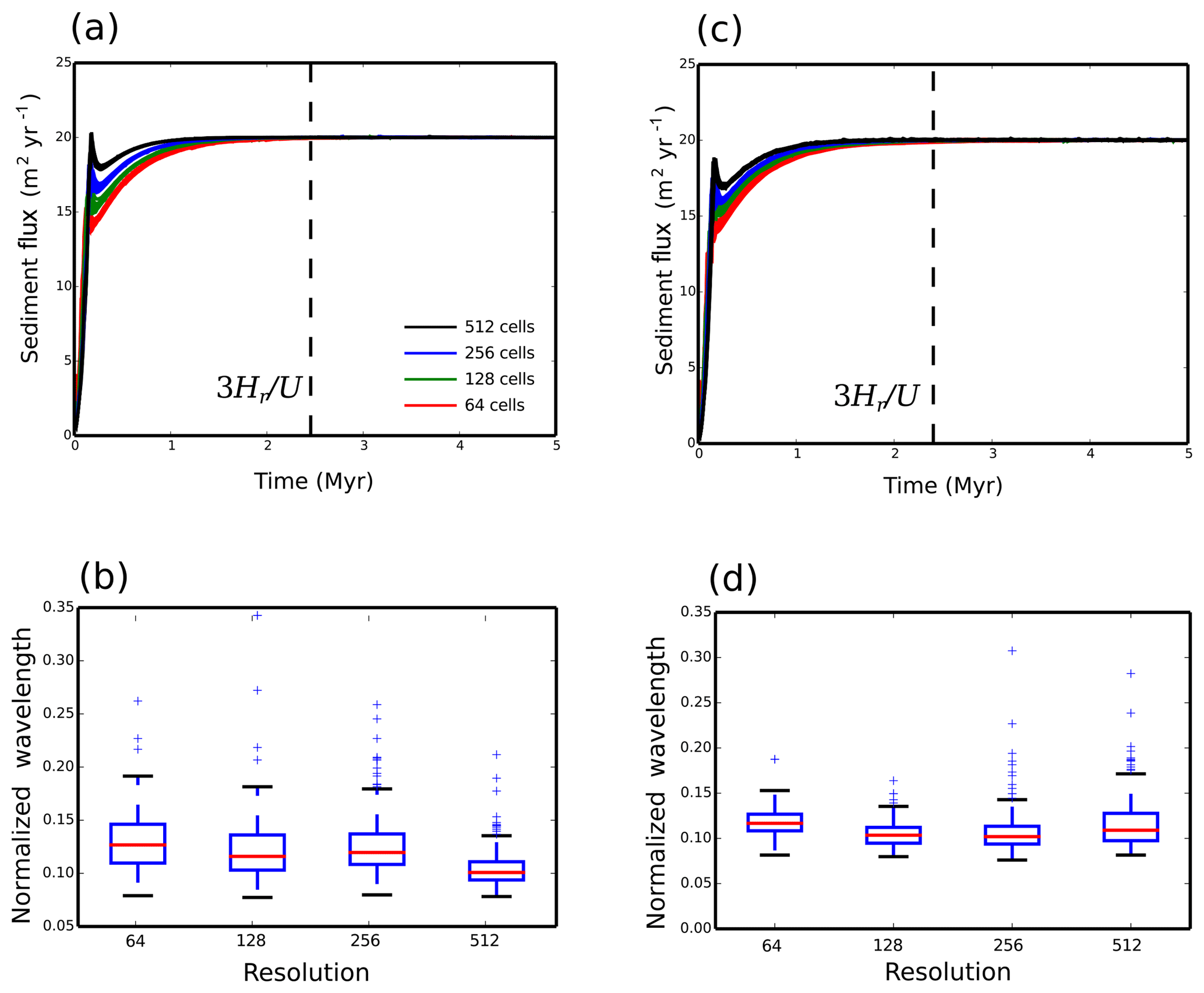
Figure 5Dimensional sediment flux that exits the model domain and box–whisker plots of the dimensionless valley-to-valley wavelength for each model for different resolutions, where the number of cells along the y axis is shown. (a) Sediment flux and (b) valley-to-valley wavelength for the cell-to-cell SFD algorithm. (c) Sediment flux and (d) valley-to-valley wavelength for the cell-to-cell MFD algorithm. The dashed line in panels (a), (c), and (e) marks the time at which erosion balances uplift, given by , where Hr is the relief height and U is the uplift rate (Howard, 1994).
To understand better how increasing resolution impacts the model evolution the total sediment flux eroded from the model domain is plotted against time, and the final valley spacing is calculated (Figs. 5 and 6). To calculate the valley spacing I take horizontal swaths of the spatial distribution of water flux. For each swath profile a peak finding algorithm (Negri and Vestri, 2017) is used to find the distance from peak to peak in water flux. This distance is then averaged over the 100 swath profiles and over 10 model runs to give the minimum, lower quartile, median, upper quartile, and maximum valley wavelength (Figs. 5 and 6).
For the cell-to-cell SFD it can be seen that the evolution of the model is resolution dependent, as the wind-up time reduces as resolution is increased from 64 to 512 cells along the y axis (Fig. 5a). Furthermore, the mean valley spacing reduces with increasing resolution (Fig. 5b). This behaviour is not ideal, as it means that model behaviour to perturbations in forcing might become resolution dependent. For the MFD wind-up times remain resolution dependent, while the mean valley spacing is similar for the four different resolutions (Fig. 5c and d).
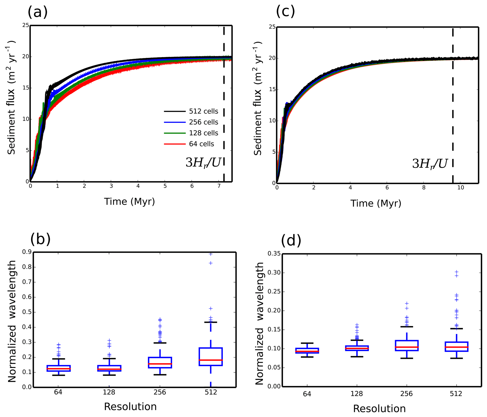
Figure 6Dimensional sediment flux that exits the model domain and box–whisker plots of the dimensionless valley-to-valley wavelength for each model for different resolutions, where the number of cells along the y axis is shown. (a) Sediment flux and (b) the node-to-node SFD algorithm. (c) Sediment flux and (d) valley-to-valley wavelength for the node-to-node MFD algorithm. The dashed line in panels (a) and (c) marks the time at which erosion balances uplift, given by , where Hr is the relief height and U is the uplift rate (Howard, 1994).
The node-to-node SFD algorithm is no better than the cell-to-cell SFD. In this case wind-up time is resolution dependent, and the valley spacing increases with increasing resolution (Fig. 6a and b). For the node-to-node SFD, at a resolution of 256 cells or less along the y axis, there is an instability in the sediment flux output. This is due to the flow tipping between adjacent nodes due to small differences in relative elevation after each time iteration. This unstable behaviour disappears for the higher resolution of 512 cells along the y axis (Fig. 6a).
It is only when node-to-node MFD is used that the LEM becomes significantly less resolution dependent (Fig. 6c and d). For the node-to-node MFD the time evolution of sediment flux is similar for all resolutions, and the valley spacing is similar as resolution is increased. The steady-state sediment flux is, however, not completely stable (Fig. 6c). This is due to the migration of the flow across the valley floors created within the model topography (Fig. 7). Even once a balance has been achieved between erosion and uplift, small lateral changes in elevation can be seen to create a negative to positive change in elevation of a few metres between time iterations, where the time step is 100 years (Fig. 7b). This is associated with an equivalent change in water flux (Fig. 7c).
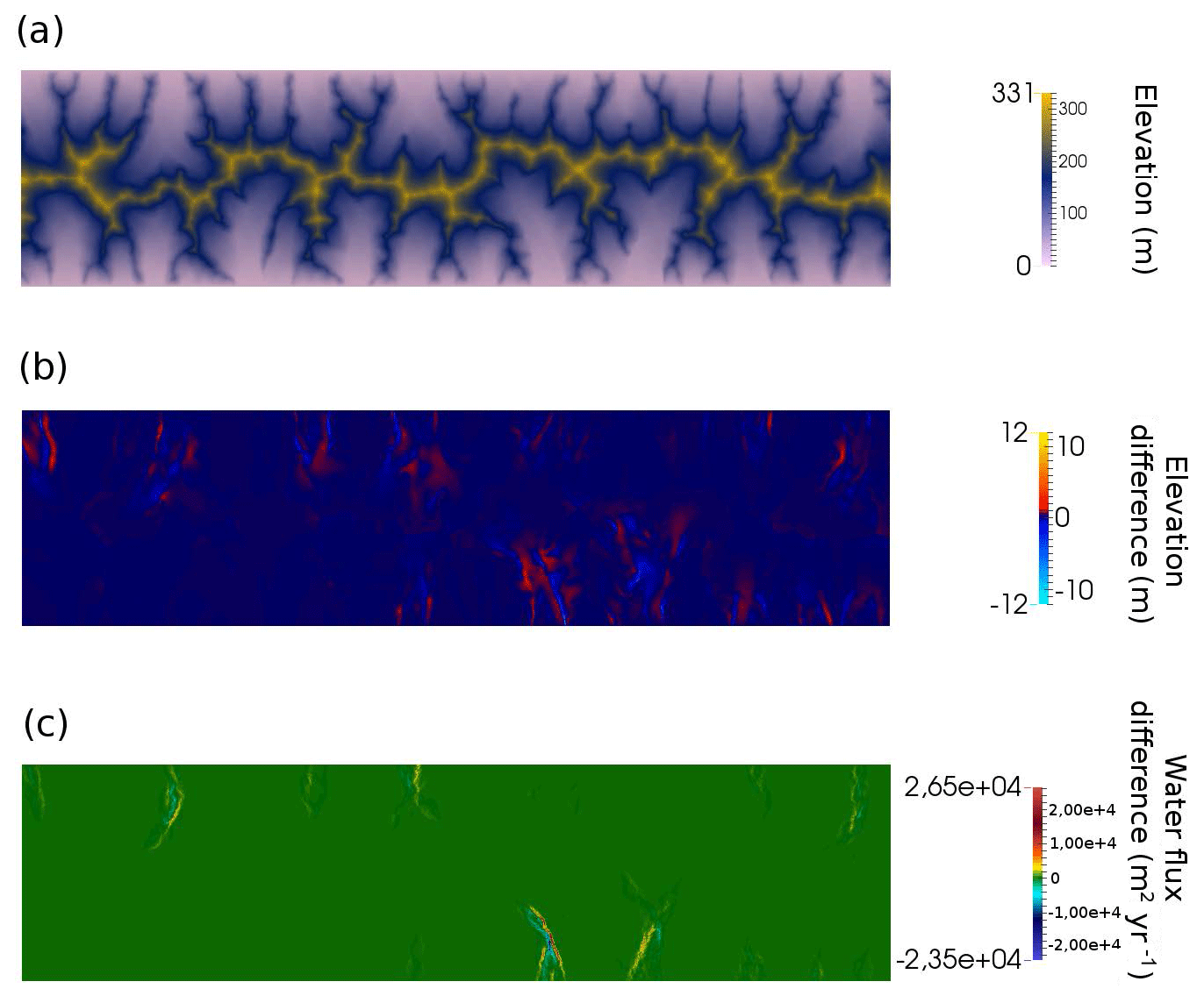
Figure 7Final steady state of an example model run for the node-to-node MFD algorithm. (a) Final model elevation where the domain is 800 km long by 100 km wide and uplift is fixed at m yr−1, the linear diffusion coefficient is κ=1 m2 yr−1, the fluvial diffusion coefficient is (m2 yr−1)n−1, and the water flux exponent is n=1.5. (b) Difference in elevation between the last two model time steps, where the time step duration is 100 years. (c) Difference in water flux between the last two model time steps.
Changing the flow routing algorithm changes the model wind-up time. This is because the rate at which the network grows and the magnitude of the water flux are affected by the choice of flow routing. The response time of the model is proportional to the water flux raised to the power n (Armitage et al., 2018). Therefore, if the drainage network forms rapidly, as is the case for cell-to-cell routing, then the model wind-up is more rapid. For the node-to-node routing, it takes longer for the network to grow (Fig. 5). Furthermore, the MFD model is the slowest to evolve to a steady state, where the total sediment flux is balanced by the uplift (Fig. 6). I have chosen to focus on n=1.5 as this value previously gave more realistic slope–area relationships at steady state (Armitage et al., 2018). However, it is interesting to note that growth of the network is a function of both the routing algorithm and the value of n.
The model that has the least resolution dependence is the node-to-node MFD (Figs. 4c and d and 6c and d). The difference between this model and the other three is that this version has the maximum possible flow directions available within my set-up. By treating flow paths as lines within the numerical grid, from any node there are six paths, which is twice as many as in the cell-to-cell MFD. This means that there is greater distribution of the flow and a reduced localizing of flow paths within the node-to-node distributed model. For SFD, increasing resolution, however, leads to multiple branches (Figs. 3b and 4b).
The grid cells in the models presented are large. At the highest resolution (2048 by 512 cells), the width of each triangle is of the order of 200 m if I was modelling a landscape 100 km wide. The model is, therefore, some approximation of local processes that give rise to the large-scale landscape. By distributing flow in multiple directions the model is in a sense approximating the hydrological processes that operate on a sub-grid-scale that give rise to the river network. The assumption of SFD is, however, too strong, and the sub-grid-scale processes are ignored.
The transport-limited model that I explore has certain limitations. In particular the valleys floors are wide and not representative of V-shaped valleys that would be expected from fluvial incision into bedrock (Fig. 4). In order to generate such valleys, a detachment-limited model, such as the stream power law, would be more appropriate. However, many stream power law models also suffer resolution dependence, as they typically use an SFD to route water (Braun and Sambridge, 1997; Braun and Willett, 2013). Pelletier (2010) looked at using MFD routing for the stream power law and found that there remained some spatial resolution dependence. The model of Pelletier (2010) used a rectangular grid and removed resolution issues by using a predictor–corrector algorithm to adjust for resolution effects. However, for the transport-limited model used here, I find that with a triangular grid the MFD routing is resolution independent without additional corrections. This is likely related to the fact that the length of each cell face is equal, while for rectangular cells the diagonal flow direction is longer than the cell faces. The implication is that for LEMs, a mesh that has cells with node-to-node spacing of equal length is preferable to a rectangular grid; however, this hypothesis will require further exploration.
MFD routing might approximate local processes that distribute flow. Another key sub-grid-scale process is the migration of drainage divides. A drainage divide is the opposite of the flow path, as it separates the valleys. The numerical model Divide And Capture (DAC) was developed to explore whether by using an analytical solution to the stream power law, the sub-grid-scale migration of drainage divides could be captured (Goren et al., 2014). DAC, therefore, uses a variant of a stream power law model; yet like the transport-limited model I present, DAC uses a triangular grid. However, DAC routes flow down the steepest route of descent (SFD). By exploring how model resolution impacts the main drainage divide, it was demonstrated that the inclusion of a sub-grid level calculation for water divides is crucial to remove otherwise spurious results (Goren et al., 2014).
By using the same set-up of a domain of 4 to 1 aspect ratio, uplift at 0.1 mm yr−1, and a precipitation rate of 1 m yr−1, I have explored how valley spacing varies as a function of resolution in the DAC model. DAC uses an adaptive mesh; therefore, the settings on how the re-meshing occurs needed to be altered to achieve an increase in the number of cells. By comparing two models at a different resolution (23 172 cells compared to 93 734), it can be seen that the median wavelength is very similar (Fig. 8).
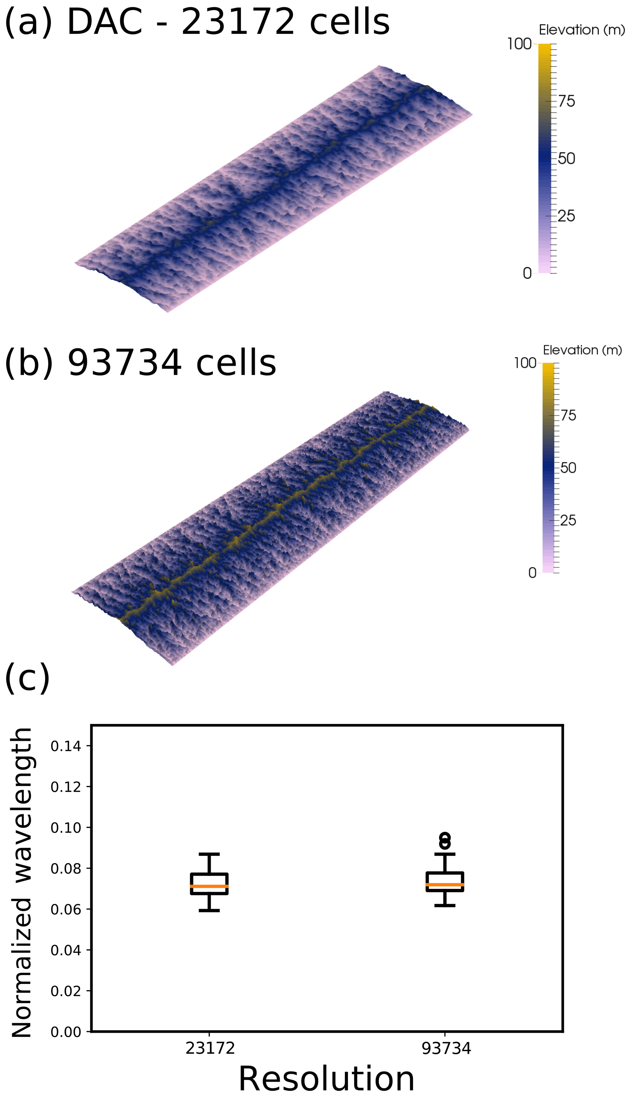
Figure 8Comparison of two model results using Divide And Capture (DAC; Goren et al., 2014) at different resolutions. (a) Model steady state for an initial resolution of 51 by 204 cells, which after adaptive re-meshing increases to 23 172 cells. (b) Model steady state for an initial resolution of 101 by 404 cells, which after adaptive re-meshing increases to 93 734 cells. (c) Comparison of the wavelength of valleys for the two models, taken from 20 swaths 1.25 km wide from the left-hand boundary (see code availability for python scripts and DAC input files).
The implication of the results I present here, and from the development of DAC, is that processes at a sub-grid level are of a crucial importance to model stability, and hence great care must be taken in generating reduced-complexity LEMs. At a small spatial and temporal scale, the landscape evolution model CAESAR-LISFLOOD (Coulthard et al., 2013), which has a rectangular grid, has been tested for different resolutions and is found to converge to the same solution at sufficiently high resolution. CAESAR-LISFLOOD uses a version of the shallow-water equations to solve for river flow, where water flows in four directions (Manhattan neighbours) and, therefore, uses an MFD rather than an SFD algorithm. Furthermore CAESAR-LISFLOOD operates on a resolution that is smaller than the width of an individual channel. This suggests that at a small spatial scales, where water depth is captured, a rectangular grid combined with an MFD algorithm is appropriate. Such a high-resolution model, however, cannot be run over periods greater than several millennia (Coulthard and van der Weil, 2013). Therefore, to explore how landscape evolves over millions of years, I suggest we must distribute flow across the model domain and use meshes of equal node-to-node spacing to avoid resolution dependence.
In experiments of sediment transport it has been noted that when the catchment outlet is fixed in time, the landscape does not achieve a steady fixed topography (Hasbergen and Paola, 2000). It has been previously suggested that this behaviour can be replicated within an LEM by introducing a distributed routing algorithm (Pelletier, 2004). This modelling result has, however, been challenged by, for example, Perron et al. (2008), where it has been suggested that distributive flow routing algorithms in fact create a fixed topography at steady state. My model, however, is in agreement with the initial findings of Pelletier (2004). It has been previously noted that an MFD algorithm will give more diffuse valley bottoms compared to an SFD algorithm (Freeman, 1991). If landscapes are indeed never steady, then perhaps this unsteady nature is due to the diffuse sediment transport across wide flood plains, which feeds up into the drainage basins. It is, after all, within the valley floor that the distributed flow routing is the most unsteady (Fig. 7c).
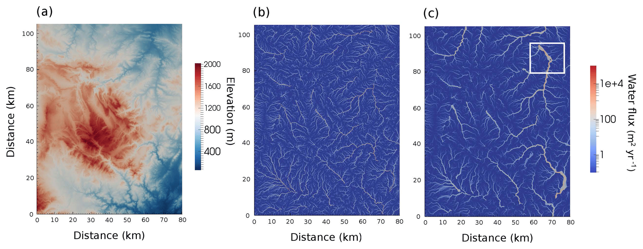
Figure 9Application of the cell-to-cell SFD and node-node MFD algorithms to a palaeo-DEM (digital elevation model). (a) Palaeo-DEM created from ASTER data of the Ebro region of Spain. (b) Water flux after 20 kyr of model evolution assuming an SFD with a model resolution of 1024×1024 cells. Uplift is assumed to be very small at 10−5 m yr−1, with a precipitation rate held constant at 0.1 m yr−1. (c) Water flux for after 20 kyr for a model assuming the node-to-node MFD routing. The white box in the top right highlights a region of the Riu Bergantes catchment where the river is known to have shifted course during the Holocene.
In nature we observe that river networks are not fixed in space and time; rather, various processes lead to changing flow directions. To further explore how realistic the cell-to-cell SFD and node-to-node MFD algorithms are, I compare how the flow of water is predicted to evolve after a 20 kyr interval. The initial condition is a palaeo-DEM generated from ASTER data from the Ebro Basin, Spain (Fig. 9a). The river valleys have been filled and the landscape has been smoothed in an attempt to approximate this landscape in the late Pleistocene. This landscape is then allowed to evolve, assuming a uniform uplift of 10−5 m yr−1 and a precipitation rate held constant at 0.1 m yr−1. I assume that (m2 yr−1)n−1, m2 yr−1, and n=1.5. Under these conditions the landscape is left to evolve for 20 kyr (Fig. 9) with zero gradient boundaries on the east, west, and southern sides and fixed elevation on the northern boundary.
The initial condition is derived from a real landscape, and as the model allows for deposition in regions of low slope, both model routing algorithms do not create drainage patterns that fully connect to the boundaries (Fig. 9b and c). This problem of too much deposition within regions of low slope, such that the water flux does not reach the model boundaries, can be overcome with the application of a “carving” algorithm. As for example applied within the TopoToolbox Landscape Evolution Model (TTLEM), a minima imposition can be used to make sure rivers keep on flowing down through regions of low slope (Campforts et al., 2017). Such an additional algorithm will, however, affect how the network grows within the model, so for this example, I have left the routing algorithm to drain internally.
Despite this imperfection, the internal drainage patterns still prove to be insightful. The cell-to-cell SFD algorithm creates single paths for the flow of water (Fig. 9b). After the 20 kyr duration, it is observed that high water flux is concentrated within the deep valleys. The node-to-node MFD algorithm creates multiple flow paths that exit the mountain valleys and migrate onto the flood plains (Fig. 9c). Field studies of the Riu Bergantes have found that this catchment has experienced periods of significant sediment reworking, potentially related to climatic change (Whitfield et al., 2013). The region outlined with the white box in Fig. 9c shows evidence of terrace formation related to lateral movement of the Riu Bergantes during the Holocene (Whitfield et al., 2013). In particular, where the flow paths create a small island (see Fig. 9c, centre of the white box), there is evidence from terrace deposits that the course of the Riu Bergantes has flipped from the eastern to the western side of this island. The cell-to-cell SFD cannot create this observed behaviour. Therefore, as well as creating landscape evolution that is not resolution dependent, the MFD algorithm creates landscape evolution that is, relative to the SFD, closer to that observed in nature.
In the study of the evolution of the earth's surface we are increasingly turning to models that attempt to capture the complexities of surface processes. It is, however, clear that many LEMs are resolution dependent (Schoorl et al., 2000). The source of this resolution dependence is the numerical methods that we employ to route surface water. Unless we model landscape evolution at a spatial scale that is smaller than an individual river, we must somehow approximate this flow. By treating flow from node to node within the model mesh and by distributing flow down these lines, the LEM developed here is no longer resolution dependent. Furthermore the model evolution is closer to what we observe. Therefore, I would strongly suggest that for LEMs that operate at a scale larger than the resolution of a river, we must use MFDs.
The code fLEM is available from the following repository: https://bitbucket.org/johnjarmitage/flem/ (Armitage, 2019a). The valley wavelength Python script and DAC input files are available from the following repository: https://bitbucket.org/johnjarmitage/dac-scripts/ (Armitage, 2019b). DAC was developed by Liran Goren; see https://gitlab.ethz.ch/esd_public/DAC_release/wikis/home (last access: 16 January 2019).
The author declares that there is no conflict of interest.
This work was inspired by a series of meetings organized by the
Facsimile working group and by a visit to the Riu Bergantes catchment in
Spain in October 2017. John Armitage is funded through the French Agence
National de la Recherche, Accueil de Chercheurs de Haut Niveau call, grant
“InterRift”. I would like to thank Kosuke Ueda and Liran Goren for help in running DAC. I would also like to thank Liran Goren and Andrew Wickert for
their reviews.
Edited by: Jean Braun
Reviewed by: Liran Goren, Andrew Wickert, and one anonymous
referee
Allen, G. H. and Pavelsky, T. M.: Global extent of rivers and streams, Science, 361, 585–588, https://doi.org/10.1126/science.aat0636, 2018. a, b
Armitage, J.: fLEM, available at: https://bitbucket.org/johnjarmitage/flem/, last access: 16 January 2019a. a
Armitage, J.: dac-scripts, available at: https://bitbucket.org/johnjarmitage/dac-scripts/, last access: 16 January 2019b. a
Armitage, J. J., Whittaker, A. C., Zakari, M., and Campforts, B.: Numerical modelling of landscape and sediment flux response to precipitation rate change, Earth Surf. Dynam., 6, 77–99, https://doi.org/10.5194/esurf-6-77-2018, 2018. a, b, c, d, e
Braun, J. and Sambridge, M.: Modelling landscape evolution on geological time scales: a new method based on irregular spatial discretization, Basin Res., 9, 27–52, 1997. a, b
Braun, J. and Willett, S. D.: A very efficient O(n), implicit and parallel method to solve the stream power equation governing fluvial incision and landscape evolution, Geomorphology, 180–181, 170–179, https://doi.org/10.1016/j.geomorph.2012.10.008, 2013. a
Campforts, B., Schwanghart, W., and Govers, G.: Accurate simulation of transient landscape evolution by eliminating numerical diffusion: the TTLEM 1.0 model, Earth Surf. Dynam., 5, 47–66, https://doi.org/10.5194/esurf-5-47-2017, 2017. a
Coulthard, T. J. and Van de Wiel, M. J.: Climate, tectonics or morphology: what signals can we see in drainage basin sediment yields?, Earth Surf. Dynam., 1, 13–27, https://doi.org/10.5194/esurf-1-13-2013, 2013. a
Coulthard, T. J., Neal, J. C., Ramirez, P. D. B., de Almedia, G. A. M., and Hancock, G. R.: Integrating the LISFLOOD-FP 2D hydrodynamic model with the CAESAR model: implications for modelling landscape evolution, Earth Surf. Proc. Land., 38, 1897–1906, https://doi.org/10.1002/esp.3478, 2013. a
Davy, P. and Lague, D.: Fluvial erosion/transport equation of landscape evolution models revisited, J. Geophys. Res.-Earth, 114, F03007, https://doi.org/10.1029/2008JF001146, 2009. a
Freeman, T. G.: Calculating catchment area with divergent flow based on a regular grid, Comput. Geosci., 17, 413–422, 1991. a
Goren, L., Willett, S. D., Herman, F., and Braun, J.: Coupled numerical-analytical approach to landscape evolution modelling, Earth Surf. Proc. Land., 39, 522–545, https://doi.org/10.1002/esp.3514, 2014. a, b, c
Granjeon, D. and Joseph, P.: Concepts and applications of a 3-D multiple lithology, diffusive model in stratigraphic modelling, in: Numerical Experiments in Stratigraphy, edited by: Harbaugh, J. W., Watney, W. L., Rankey, E. C., Slingerland, R., and Goldstein, R. H., Society for Sedimentary Geology, 62, Special Publications, 197–210, 1999. a
Hasbergen, L. E. and Paola, C.: Landscape instability in an experimental drainage basin, Geology, 28, 1067–1070, 2000. a
Howard, A.: A detachment-limited model of drainage basin evolution, Water Resour. Res., 30, 2261–2285, 1994. a, b
Kooi, H. and Beaumont, C.: Escarpment evolution on high-elevated rifted margins; insights derived from a surface-processes model that combines diffusion, advection and reaction, J. Geophys. Res., 99, 12191–12209, 1994. a
Negri, L. H. and Vestri, C.: peakutils: v1.1.0, https://doi.org/10.5281/zenodo.887917, 2017. a
Pelletier, J. D.: Persistent drainage migration in a numerical landscape evolution model, Geophys. Res. Lett., 31, L20501, https://doi.org/10.1029/2004GL020802, 2004. a, b, c
Pelletier, J. D.: Minimizing the grid-resolution dependence of flow-routing algorithms for geomorphic applications, Geomorphology, 122, 91–98, https://doi.org/10.1016/j.geomorph.2010.06.001, 2010. a, b
Perron, J. T., Dietrich, W. E., and Kirchner, J. W.: Controls on the spacing of first-order valleys, J. Geophys. Res., 113, F04061, https://doi.org/10.1029/2007JF000977, 2008. a, b, c
Salles, T., Flament, N., and Muller, D.: Influence of mantle flow on the drainage of eastern Australia since the Jurasic Period, Geochem. Geophy. Geosy., 18, 280–305, https://doi.org/10.1002/2016GC006617, 2017. a
Schoorl, J. M., Sonneveld, M. P. W., and Veldkamp, A.: Three-dimensional landscape process modelling: the effect of DEM resolution, Earth Surf. Proc. Land., 25, 1025–1034, 2000. a, b, c, d
Simpson, G. and Schlunegger, F.: Topographic evolution and morphology of surfaces evolving in response to coupled fluvial and hillslope sediment transport, J. Geophys. Res., 108, 2300, https://doi.org/10.1029/2002JB002162, 2003. a, b, c
Smith, T. R. and Bretherton, F. P.: Stability and conservation of mass in drainage basin evolution, Water Resour. Res., 8, 1506–1529, https://doi.org/10.1029/WR008i006p01506, 1972. a
Syvitski, J. P. and Milliman, J. D.: Geology, geography, and humans battle for dominance over the delivery of fluvial sediment to the coastal ocean, J. Geol., 115, 1–19, https://doi.org/10.1086/509246, 2007. a
Temme, A. J. A. M., Armitage, J. J., Attal, M., van Gorp, W., Coulthard, T. J., and Schoorl, J. M.: Choosing and using landscape evolution models to inform field stratigraphy and landscape reconstruction studies, Earth Surf. Proc. Land., 42, 2167–2183, https://doi.org/10.1002/esp.4162, 2017. a
Whitfield, R. G., Macklin, M. G., Brewer, P. A., Lang, A., Mauz, B., and Whitfield, E.: The nature, timing and controls of the Quaternary development of the Rio Bergantes, Ebro basin, northeast Spain, Geomorphology, 196, 106–121, https://doi.org/10.1016/j.geomorph.2012.04.014, 2013. a, b