the Creative Commons Attribution 4.0 License.
the Creative Commons Attribution 4.0 License.
 | 26 Aug 2019
Inferring the timing of abandonment of aggraded alluvial surfaces dated with cosmogenic nuclides
Mitch K. D'Arcy
Taylor F. Schildgen
Jens M. Turowski
Pedro DiNezio
Information about past climate, tectonics, and landscape evolution is often obtained by dating geomorphic surfaces comprising deposited or aggraded material, e.g. fluvial fill terraces, alluvial fans, volcanic flows, or glacial till. Although surface ages can provide valuable information about these landforms, they can only constrain the period of active deposition of surface material, which may span a significant period of time in the case of alluvial landforms. In contrast, surface abandonment often occurs abruptly and coincides with important events like drainage reorganization, climate change, or landscape uplift. However, abandonment cannot be directly dated because it represents a cessation in the deposition of dateable material. In this study, we present a new approach to inferring when a surface was likely abandoned using exposure ages derived from in situ-produced cosmogenic nuclides. We use artificial data to measure the discrepancy between the youngest age randomly obtained from a surface and the true timing of surface abandonment. Our analyses simulate surface dating scenarios with variable durations of surface formation and variable numbers of exposure ages from sampled boulders. From our artificial data, we derive a set of probabilistic equations and a MATLAB tool that can be applied to a set of real sampled surface ages to estimate the probable period of time within which abandonment is likely to have occurred. Our new approach to constraining surface abandonment has applications for geomorphological studies that relate surface ages to tectonic deformation, past climate, or the rates of surface processes.
- Article
(4736 KB) - Full-text XML
-
Supplement
(788 KB) - BibTeX
- EndNote


Geomorphological studies that link the formation of landforms to past changes in climate or tectonic deformation depend on the accurate dating of surfaces comprising aggraded or deposited material. Surfaces commonly targeted for dating include alluvial fans, fluvial fill terraces, glacial till, pediments, and volcanic flows, among others. For example, the ages of fluvial fill terraces and alluvial-fan surfaces have been used to (i) decipher how erosion and sedimentation have responded to past hydroclimate changes (Owen et al., 2014; Schildgen et al., 2016; Tofelde et al., 2017); (ii) derive time-integrated slip rates for active faults (e.g. Frankel et al., 2007, 2011; Gosse, 2011; Hughes et al., 2018); and (iii) quantify the rates of surface processes such as weathering, landform erosion, or channel avulsion and incision (Schildgen et al., 2012; Regmi et al., 2014; Bufe et al., 2017; D'Arcy et al., 2018).
A common assumption is that a geomorphic surface can be represented by a single formation age. Surfaces are usually point-sampled and dated in multiple locations, e.g. by cosmogenic nuclide exposure dating of surface boulders. Typically, sampling is limited to a small number of (often fewer than 10) large, stable surface boulders, which exhibit no evidence of weathering, rotation, or disturbance. From the set of exposure ages obtained, an average surface age can be calculated with an uncertainty that reflects both analytical uncertainty and the spread of sampled ages. However, many geomorphic surfaces are active for an extended period of time, during which material is continually deposited until the surface is abandoned (e.g. Savi et al., 2016; Denn et al., 2017; Foster et al., 2017). Alluvial-fan surfaces provide one example. Rather than being formed instantaneously, fan surfaces are typically active for thousands or tens of thousands of years before being abandoned when the channel avulses or incises (e.g. Dühnforth et al., 2007). This prolonged period of activity results in a meaningful spread in ages collected from a single surface (e.g. Owen et al., 2011). For any geomorphic surface with a non-negligible period of formation, a set of surface ages will capture a portion of the full time span over which that surface was active. An average of those ages will sit somewhere within the true time span of surface deposition, whereas the maximum age might approximate the onset of surface activity, and the minimum age might approximate the timing of surface abandonment.
In some cases, the timing of surface abandonment may be a more useful constraint than an average surface age. In contrast to surface deposition, abandonment occurs at a particular moment in time (e.g. coinciding with a switch to incision) and so can, in principle, be defined with greater precision. For surfaces with an extended period of formation, the timing of abandonment is more likely to coincide with events of interest such as reorganization of a drainage network (Bufe et al., 2017); changes in climate, sediment supply, or base level (Steffen et al., 2009; Tofelde et al., 2017; Mouslopoulou et al., 2017; Brooke et al., 2018); or tectonic deformation such as faulting, uplift, or subsidence (e.g. Frankel et al., 2007, 2011; Ganev et al., 2010). Abandonment ages would also benefit any study that uses surface exposure dating to measure the rates of post-depositional processes, such as in situ weathering (e.g. White et al., 1996, 2005; D'Arcy et al., 2015, 2018), the topographic decay of landforms (e.g. Hanks et al., 1984; Andrews and Bucknam, 1987; Spelz et al., 2008), or channel avulsion and incision (e.g. Schildgen et al., 2012; Finnegan et al., 2014; Malatesta et al., 2017). Yet the abandonment of a surface represents a cessation in the deposition of dateable material, and therefore cannot be directly dated. Instead, the timing of abandonment must be inferred. Some studies make assumptions about when geomorphic surfaces were abandoned based on independent information such as palaeoclimate records (e.g. Macklin et al., 2002; Cesta and Ward, 2016); others assume that the youngest sampled surface ages fall close to the timing of surface abandonment (e.g. Sarıkaya et al., 2015; Foster et al., 2017; Ratnayaka et al., 2018; Clow et al., 2019). These assumptions risk interpretations that are circular (in the former case) or potentially inaccurate (in the latter case), highlighting the need for a robust method to quantitatively infer the timing of surface abandonment from a set of sampled surface ages.
Here, we introduce a new probabilistic approach to constraining when a depositional surface was abandoned based on what is known about its activity. We use artificial data to randomly point-sample the ages of virtual surfaces in scenarios that are representative of studies dating natural geomorphic landforms such as alluvial fans. We quantify how close the youngest obtained age is likely to fall within the true timing of abandonment, depending on the overall period of surface activity and the number of samples collected. From these artificial data, we derive a set of probabilistic equations and a MATLAB tool that can be applied to real geomorphic surfaces to estimate when they were abandoned. Finally, we demonstrate the application of these equations and the MATLAB tool to natural surfaces with a case study of dated alluvial-fan surfaces in Baja California, Mexico.
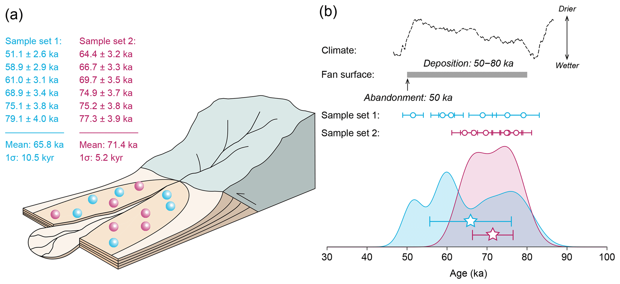
Figure 1(a) Conceptual alluvial-fan surface that was formed over a 30 kyr period, from 80 to 50 ka, after which it was abandoned, e.g. due to incision. Two different dating scenarios (sample sets 1 and 2) are shown in which six surface ages are randomly selected. (b) The true period of surface activity (grey bar) compared with the sampled ages presented as data points (circles), kernel density plots, and mean surface ages ±1 standard deviation (stars). A hypothetical climate scenario is depicted as a dotted line.
Here, we present a hypothetical example of a dated alluvial-fan surface to illustrate why the timing of abandonment may, in some cases, be more useful than an average of sampled surface ages. Consider an alluvial-fan surface that was active for a 30 kyr time span, starting at 80 ka and ending at 50 ka, when the surface was abandoned due to fan incision (Fig. 1). In this example, deposition occurred on the fan surface throughout a period of climatic stability and abandoned when the climate changed, and we make the assumption that there is an equal likelihood of obtaining any age within the entire period of deposition. A distribution of surface ages can be obtained by point-sampling the fan surface; an approach analogous to studies that measure the exposure ages of boulders atop landforms. We present two arbitrarily selected possible outcomes in Fig. 1, where six surface ages are obtained. In scenario 1, the ages are distributed relatively evenly through time, producing a mean age of 65.8 ka, which closely approximates the true average surface age of 65 ka, with a standard deviation of 10.5 kyr. In scenario 2, the ages obtained are unevenly distributed through time, producing a slightly older mean surface age (71.4 ka) and a smaller standard deviation (5.2 kyr). These scenarios are plotted against time in Fig. 1b as data points and kernel density plots, and they resemble equivalent natural datasets (e.g. Owen et al., 2014).
Sample set 2 is more tightly clustered than sample set 1, despite being less representative of the average surface age, illustrating that greater clustering of ages is not necessarily an indicator of accuracy. Furthermore, neither average age corresponds to any meaningful event. The fan surface was equally active for the entire period between 80 and 50 ka, the average ages sit within a period of climatic and depositional stability, and the peaks in the kernel density plots are artefacts created by randomly sampling a linear series.
In contrast, the abandonment of the fan surface does occur at a precise moment in time when deposition ends at 50 ka. In this example, abandonment coincides with an abrupt change in climate that triggered an incision event (cf., Simpson and Castelltort, 2012), so it is arguably a more informative target for dating than an average age that imprecisely approximates the mid-point in the duration of surface deposition. However, the abandonment of the surface represents a cessation in the deposition of dateable material, so its timing instead must be inferred from what is known about the surface activity. Given that (i) the sampled ages constrain the time span over which the surface was formed and (ii) abandonment occurred sometime after the youngest age, it could be assumed that the youngest sampled age best approximates abandonment. In scenario 1, the youngest age falls within ∼1 kyr of surface abandonment, which would enable a correct interpretation of correlation between fan incision and the climate change event. In scenario 2, however, there is a ∼14 kyr discrepancy between the youngest sampled age and the timing of surface abandonment, which would probably fail to demonstrate the correlation between climate change and fan incision. Therefore, the question becomes the following: how close is the youngest age obtained from a surface to the actual timing of surface abandonment?
This question cannot currently be answered for a natural dataset, yet the ability to reliably estimate when a surface was abandoned has important implications for many geomorphological applications (see Sect. 1). In this study, we use artificial data to simulate natural surfaces that undergo active deposition over variable periods of time and dated with a limited number of surface ages. These artificial data are analogous to studies that date natural geomorphic surfaces, for example, with cosmogenic nuclide exposure ages obtained from sampled boulders on alluvial fans or fluvial fill terraces. However, unlike field-based datasets, artificial data enable us to constrain the time difference between the youngest age obtained from a geomorphic surface and the true timing of surface abandonment, which is generally unknowable for natural surfaces. There are several additional advantages to taking an artificial-data approach. First, we can repeat the random sampling of surface ages (e.g. as depicted in Fig. 1) many times to probabilistically determine where the youngest sampled age tends to fall with respect to abandonment. Second, we can prescribe the surface parameters, meaning the exact timing of abandonment and the full period of surface activity are known. Third, we can select surface properties that are representative of natural geomorphic surfaces and numbers of samples commonly obtained in geomorphic studies. Fourth, we can perform a thorough quantification of the uncertainties in our analyses. For the above reasons, the artificial-data approach allows us to derive a set of equations and develop a MATLAB tool that can then be applied to natural datasets (a set of surface ages) to determine the probability of surface abandonment occurring within a specified window of time.
3.1 Artificial-data approach
We used artificial data to constrain the temporal discrepancy, which we denote τ, between the youngest age sampled on a surface (amin) and the actual timing of surface abandonment (taban):
Our experiments are designed to be representative of natural alluvial-fan surfaces but the results are more widely applicable to any abandoned depositional surface that has been dated.
In the absence of additional information (e.g. the existence of an independent constraint, such as a younger alluvial-fan surface with an intermediate age), the abandonment of a surface could have occurred at any time between the youngest sampled age, amin, and the present, or within a particular time window after amin. In the example case (Fig. 1), the data in sample set 1 would require a time window, τ, of 1.1 kyr placed immediately after the youngest age to overlap with the correct timing of surface abandonment, taban. However, for sample set 2, a 14.4 kyr window is required. For natural cases, the abandonment timing is unknown; we know the temporal discrepancy between amin and taban in these artificial-data examples because we impose taban. An advantage of the artificial-data approach is that knowledge of taban allows us to quantify τ in every tested scenario, which in turn enables us to determine probability distributions of τ. Conceptually, the size or τ, i.e. the proximity of amin to taban, depends on the number of surface ages obtained, n. The greater the number of samples, the closer the youngest sampled age is likely to come to the abandonment age (Fig. 2a). The size of τ also depends on the total duration of surface activity, which we denote as T. If n ages are randomly sampled from a longer time span, T, then amin is likely to fall farther from taban (Fig. 2b).
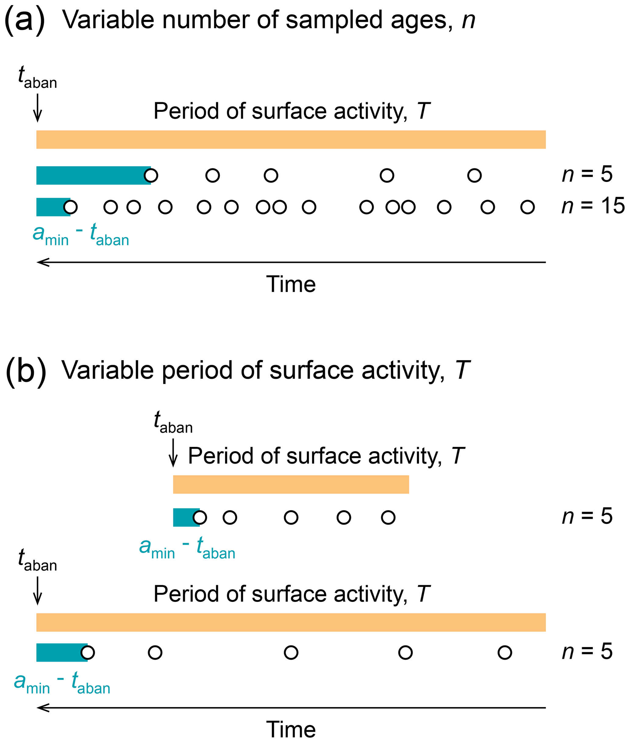
Figure 2Schematic surface with a period of activity, T (orange bar), abandoned at taban, and randomly sampled with n ages (circles). (a) If n increases, the youngest sampled age, amin, is likely to fall closer to taban. (b) If T increases, the youngest sampled age, amin, is likely to fall farther from taban, even if the same number of ages are sampled.
Our artificial-data experiments simulate surfaces with durations of activity, T, between 10 and 50 kyr, sampled with numbers of surface ages, n, between 2 and 10. These values are representative of natural alluvial-fan surfaces and typical dating studies involving a small number of ages. For each combination of T and n, we randomly sampled a set of surface ages 10 000 times, allowing us to constrain the probability that amin falls within a certain temporal window (τ) of taban in each scenario.
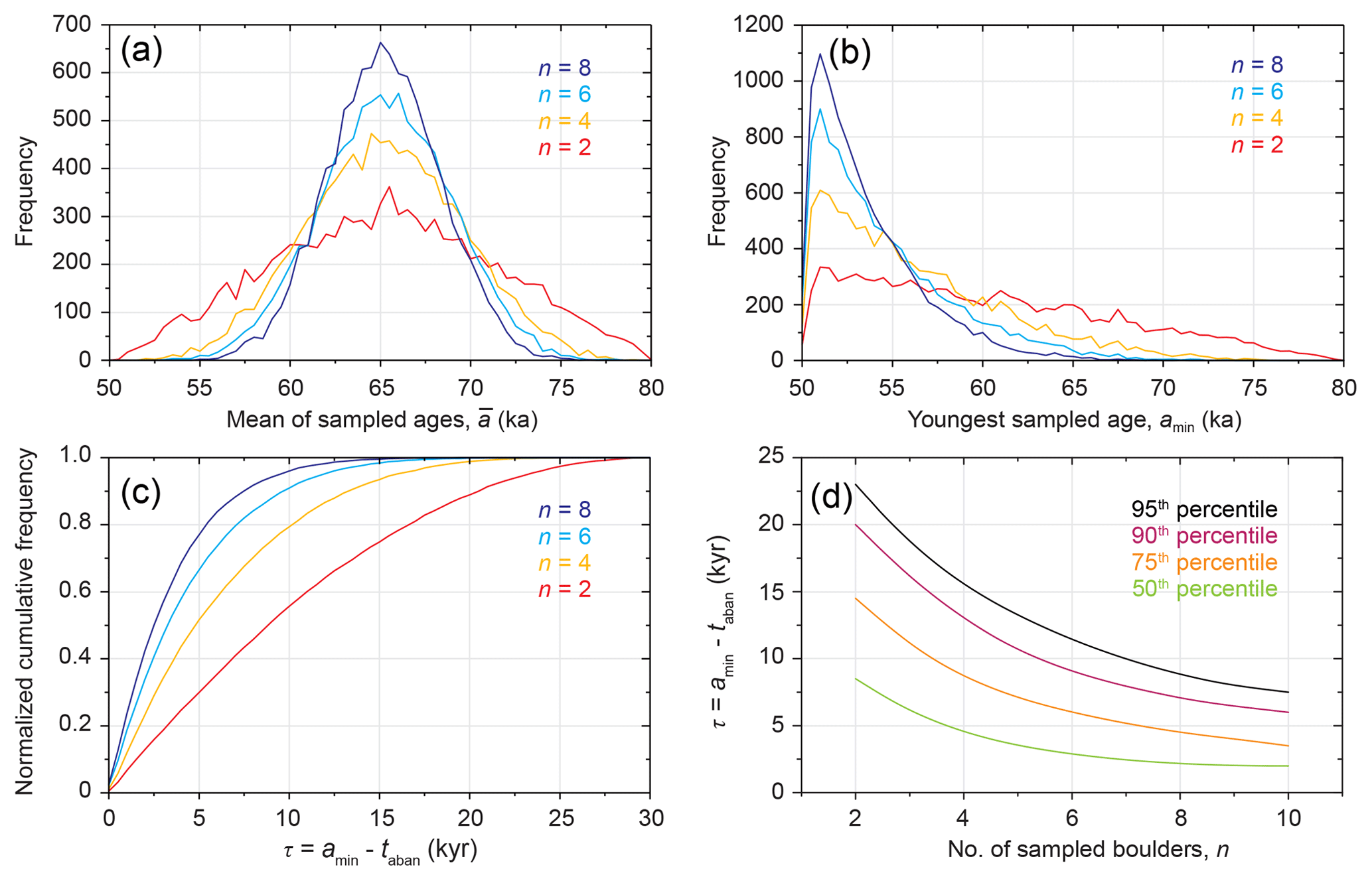
Figure 3Example results of the artificial-data experiments for a surface active from 80 to 50 ka (T=30 kyr). A number of ages, n, were randomly sampled from the surface 10 000 times. (a) Frequency distributions of resulting mean sampled age, . (b) Frequency distributions of the youngest sampled age, amin. (c) Cumulative frequency distributions of τ normalized to a sum of 1. (d) Selected percentiles of τ plotted against n.
3.2 Implementation
We first implemented our experiments using discrete sampling within a spreadsheet. For each surface, we created a list of selectable surface ages spanning the total period of surface activity, T, and placed at equal intervals of 0.1 kyr. For the example case (Fig. 1), this would mean a list of selectable ages of 80.0, 79.9, 79.8 ka, etc., to a minimum value of 50.0 ka. We chose periods of surface activity, T, equal to 10, 20, 30, 40, and 50 kyr. From each list, we randomly selected n unique values and repeated this exercise 10 000 times for each integer value of n between 2 and 10. For example, if n=6 and T=20 kyr, then we extracted 10 000 different datasets, each comprising six randomly selected ages, from the 20 kyr long list of selectable ages available at 0.1 kyr intervals. This process is analogous to random sampling of six boulders for cosmogenic nuclide exposure dating on an alluvial-fan surface that formed over a 20 kyr period and deposited a selectable boulder once every 100 years. We extracted 10 000 sets of ages for each of the 45 different combinations of T (five unique values) and n (nine unique values). For each dataset, we calculated the mean value of the selected ages, , and the time difference between the youngest age and the abandonment time, τ. We then determined cumulative frequency distributions of τ in each scenario with a given combination of T and n.
To test whether 10 000 iterations are sufficient to produce reliable statistics and whether the discretization of ages has an important effect, we repeated all our artificial-data experiments using a non-discrete approach in a MATLAB script. We defined T as a time range, from within which any point in time could be randomly sampled, i.e. tens of thousands of “selectable” surface ages were available rather than hundreds of discrete values. Performing 100 000 iterations with the MATLAB script produced results that are indistinguishable from the discrete spreadsheet-based approach with 10 000 iterations. All data analyses are provided by D'Arcy et al. (2019) in an online data repository. Finally, we explore the assumptions and limitations of our analyses in Sect. 5.3.
3.3 Experimental assumptions
In designing our artificial-data experiments, we make several assumptions. First, surface ages are randomly selected from the total period of surface activity. Therefore, when constructing our experiments, we assume that when ages are obtained from real geomorphic surfaces, they are randomly point-sampling the full time span of surface formation, and that this time span represents a uniform probability distribution of selectable ages. A uniform probability of ages may not be realistic in certain natural cases, for example, if boulders on an alluvial-fan surface are spatially clustered by age and all samples are taken from one part of the surface. Second, the entire period of surface activity is assumed to be available for sampling, i.e. no subset of the surface history is missing as a result of processes like burial or erosion. Third, all selectable ages within the period of surface activity have an equal likelihood of being sampled; this implies that the surface formed with a constant deposition rate and there are no pulses of activity that increase the probability of sampling a particular age. Finally, we do not explicitly factor in processes like nuclide inheritance, erosion, or incomplete exposure, which can affect exposure ages derived from cosmogenic nuclides. We consider the implications of all these assumptions for natural datasets in Sect. 5.3.
4.1 Random sampling of surface ages
To illustrate the results of our experiments, we first present one artificial-data scenario in Fig. 3 in which the surface is formed between 80 and 50 ka (i.e. T=30 kyr) and is randomly sampled with , 6, or 8 ages (with 10 000 repeat experiments for each value of n). Figure 3a shows how a frequency distribution of the mean value of all sampled ages, , changes with n. The distribution is centred on the true average surface age of 65 ka and narrows as a greater number of ages are sampled. If only two ages are sampled, then can occupy almost any age within the full period of surface activity. As n increases, tends to fall closer to 65 ka. The distribution of approaches a normal distribution as n increases. This observation is compatible with the central limit theorem and the law of large numbers: converges on the true average surface age as the number of samples increases, despite the dataset randomly sampling a linear series.
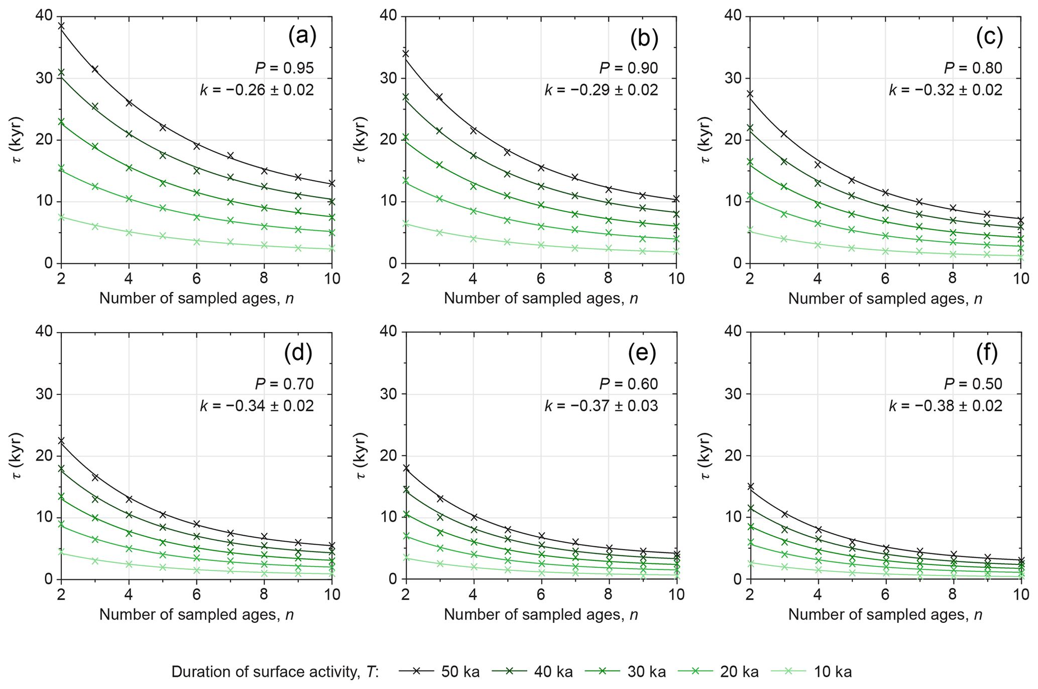
Figure 4The probable abandonment window, τ, as a function of the number of boulder ages, n. Data are shown for different probabilities, P (panels), and durations of surface activity, T (colours). Parameter k is a decay constant that depends on P (see text for details).
A frequency distribution can also be plotted for the youngest age, amin, randomly selected from the surface (Fig. 3b). If only two ages are obtained, then the youngest can fall almost anywhere between 50 and 80 ka, although the distribution is asymmetric and younger values of amin occur slightly more frequently than older values. As n increases, the distribution of amin shifts towards 50 ka such that when n=8, amin falls within 5–10 kyr of taban (i.e. τ is equal to 5–10 kyr) in the majority of sampling experiments. Cumulative frequency distributions of τ reveal how close the youngest sampled age comes to the known timing of surface abandonment (Fig. 3c). For example, if only two ages are obtained, then in 60 % of experiments, τ≤12 kyr, i.e. the youngest age falls somewhere within 12 kyr of abandonment. If six ages are obtained, then in 90 % of experiments, τ≤10 kyr. Any percentile of τ can be measured from Fig. 3c, allowing τ to be plotted against n (Fig. 3d). As a greater number of ages are obtained, the value of τ associated with a given percentile decreases, i.e. the youngest sampled age comes closer to the timing of surface abandonment. However, the decrease in τ is non-linear and diminishes with increasing n. For example, as n increases from two to four ages, the 95th percentile of τ falls from ∼23 to ∼16 kyr, but collecting another two ages (n=6) only reduces τ to ∼12 kyr. The 95th percentile of τ falls below 10 kyr when n exceeds seven ages. In other words, if seven ages are randomly sampled from a surface, abandonment will have occurred within 10 kyr after the youngest age in 95 % of cases.
We equate the percentiles of τ in Fig. 3c with the probability, P, of abandonment occurring within a time window defined by τ. Thus, if P=0.9, the window of time τ (placed immediately after amin) is large enough that in 90 % of our experiments, the true timing of surface abandonment would fall within it. This is equal to the 90th percentile of τ, which would be 7.5 kyr for the scenario T=30 kyr and n=8, for example (Fig. 3d). Note that in this scenario, τ does not imply that the surface was abandoned exactly 7.5 kyr after amin, but rather that there is a 90 % likelihood that abandonment occurred anywhere within a 7.5 kyr window after amin. The probable window of abandonment, τ, increases with P because a larger window of time is required to capture the true timing of abandonment in a greater proportion of cases.
At the same time, τ is inversely and non-linearly related to the sample size of ages obtained, n (Fig. 4). The dependencies between τ and n, T, and P are illustrated in Fig. 4 for all tested scenarios that are representative of natural alluvial-fan surfaces (n=2 to 10; T=10 to 50 kyr), with probabilities between 0.50 and 0.95. For example, if six ages are obtained from a surface that formed over a 30 kyr duration, then τ=12 kyr for P=0.95 (Fig. 4a). In other words, in 95 % of cases the youngest of six ages obtained from such a surface will fall within 12 kyr of the true timing of abandonment. Only in 5 % of cases does the discrepancy between amin and abandonment exceed 12 kyr. If P decreases to 0.5 (Fig. 4f), then τ decreases to 3 kyr for this particular scenario (n=6 and T=30 kyr).
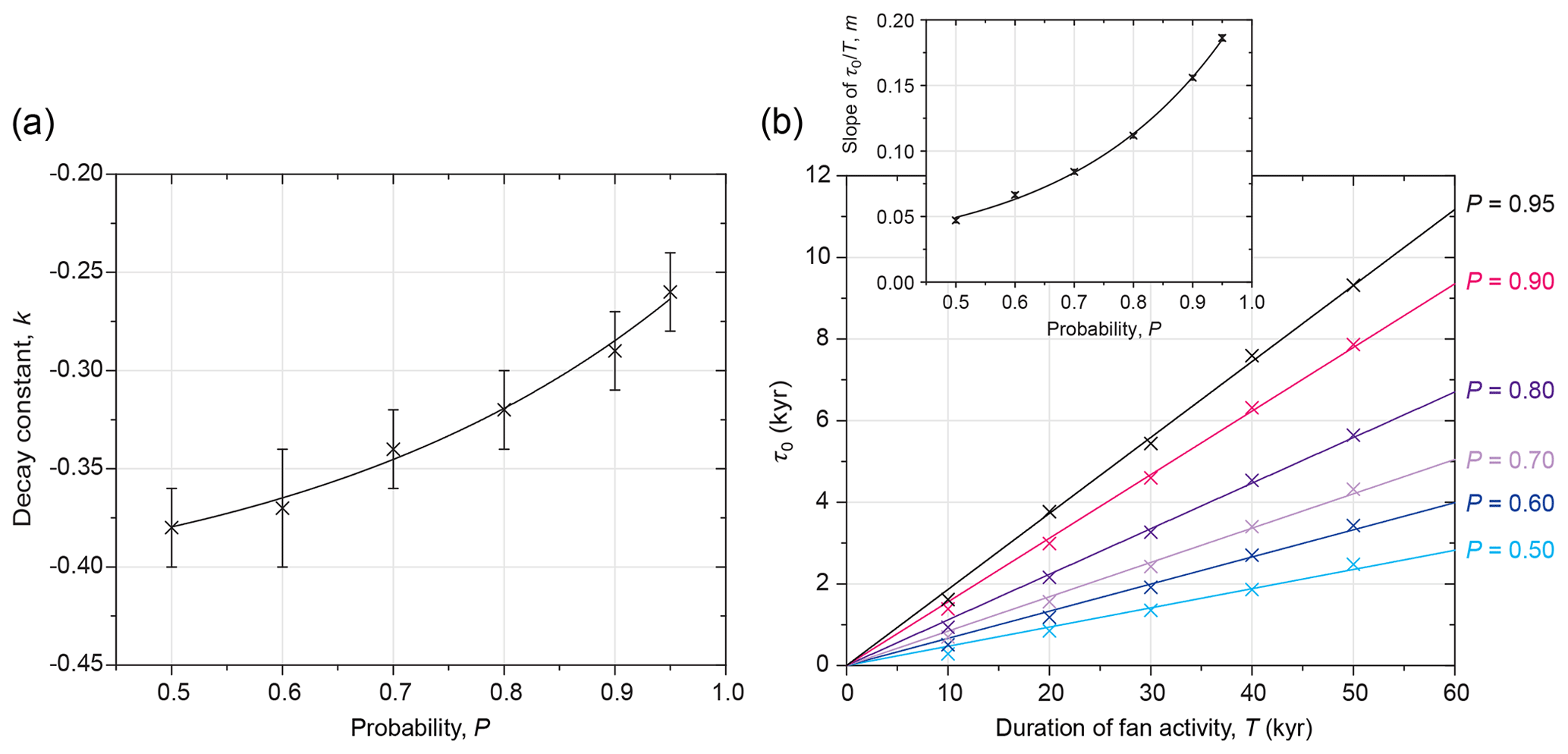
Figure 5(a) Variation in the decay constant, k, as a function of the probability, P. Error bars show the standard error in k when Eq. (2) is fitted to the data in Fig. 4. The regression corresponds to Eq. (3). (b) Variation in τ0 as a function of T for different values of P (indicated by colours). Linear regressions are fitted corresponding to Eq. (4). Inset: variation in m as a function of P. An exponential regression is fitted corresponding to Eq. (5).
The results of our artificial-data experiments (Fig. 4) can be described by one equation that allows τ to be calculated for any scenario:
Here, the parameter k is a decay constant with a negative value that increases exponentially with P (Fig. 5a):
Constants a, b, and c can be derived empirically using our artificial data. Note that we calibrate all our equations with time in kiloyears (kyr).
, ,
The parameter τ0 increases linearly with T, but with a slope that increases exponentially with P (Fig. 5b), and can therefore be described by a pair of relationships:
Parameters m0, g, and h are constants with values again determined empirically from our artificial-data experiments:
Given that τ0 signifies the value of τ as n tends towards infinity, it represents the limit of precision that can be obtained on the abandonment period, τ, when inferring the timing of surface abandonment with this probabilistic method. For the scenarios shown in Fig. 5b, which represent reasonable values of T for natural alluvial fans and desirable values of P, τ0 varies from a few centuries to ∼10 kyr.
4.2 Total period of surface formation
Equation (2) can be solved for τ (using the parameterization of Eqs. 3 through 5) with knowledge of only the number of ages sampled, n, and the total period of surface formation, T, as well as a chosen probability, P. We are able to parameterize τ using artificial data because we know the value of T in our experiments. However, when sampling natural depositional surfaces, T is unknown and instead only the span of sampled ages, amax−amin, can be measured. This span might approximate T, but some fraction of time will not be captured. Fortunately, our artificial-data experiments also allow us to determine what fraction of T is captured by amax−amin in scenarios of varying n (Fig. 6).
The artificial data indicate that, for example, six randomly distributed ages will span ∼70 % of the total time span of surface activity, T, in the average case. In the 1 % of worst (most clustered age) cases, amax−amin will only represent ∼30 % of T, and in the 1 % of best (least clustered age) cases it will represent more than 95 % of T. In half of all experiments for n=6 (from P25 to P75), amax−amin falls within 60 %–85 % of T. There is a diminishing improvement with an increasing number of sampled ages, such that by n=10 the average span of ages has only increased to ∼80 % of T and 50 % of all experiments fall between 75 % and 90 % of T. An order of magnitude more ages (hundreds) would be needed for the mean amax−amin to come within 95 % of the full period of surface activity.
A regression can be fitted to the distributions in Fig. 6, taking the form
Parameters q, r, and s are empirical coefficients derived graphically from our artificial data. For the mean case (the solid black line in Fig. 6), they take the values
Equation (6) is also fitted to ±1 standard deviation (σ) above and below the mean values in Fig. 6 (dashed black lines). For 1σ above the mean, parameters q, r, and s take the values
For 1σ below the mean, parameters q, r, and s take the values
Equation (6) can therefore be used to estimate the size of T in the average case ±1σ bounds, given the measured span of ages collected from a surface. Equations (2) through (6) are thus calibrated using our artificial data, and can be used to probabilistically calculate the window of time during which any dated surface was likely abandoned.
4.3 Application to measured surface ages
Given that Eqs. (2) through (6) are probabilistic (i.e. P is a variable), our artificial-data approach can be used to infer a probability distribution of abandonment ages from a set of measured surface ages. We illustrate the steps involved in applying Eqs. (2) through (6) and the MATLAB script to real data in Fig. 7.

Figure 6Box plots showing the fraction of the total period of fan activity, T, captured by the span of sampled boulder ages in the artificial-data experiments, amax−amin plotted against the number of sampled ages, n. Each box represents 10 000 experiments. As a greater number of ages are sampled, the span of the set of ages is more likely to capture a greater fraction of T, although with diminishing returns for increasing n. Black lines show exponential regressions corresponding to Eq. (6) and fitted to the mean values (solid) and ±1 standard deviation (dashed).
To solve for τ at a discrete probability value (P), T is first calculated with Eq. (6) and τ is then calculated using Eq. (2), with parameters defined in Eqs. (3) through (5) (Fig. 7a). These discrete values of τ can be converted into a probability distribution by calculating the density of P within fixed increments of τ. For example, in Fig. 7a, 50 % of the probability of abandonment falls within a relatively small window of time (the light blue bar for P=0.5), whereas a longer window of time is required to contain an additional 45 % of the probability of abandonment (the light pink bar for P=0.95). Thus, the density of P is greater within the window τ for P=0.5, and this density diminishes as τ and P increase. The MATLAB script (provided in the Supplement) enables determination of the continuous probability distribution of τ. After generating artificial data based on n ages and a duration of deposition T (from Eq. 6), the script calculates the density of P within fixed increments of τ. If the sampled surface ages are known with exact precision, then the resulting distribution of τ values provides a probability distribution of times that directly postdate the youngest age and yield a probability distribution of surface-abandonment ages (Fig. 7a).
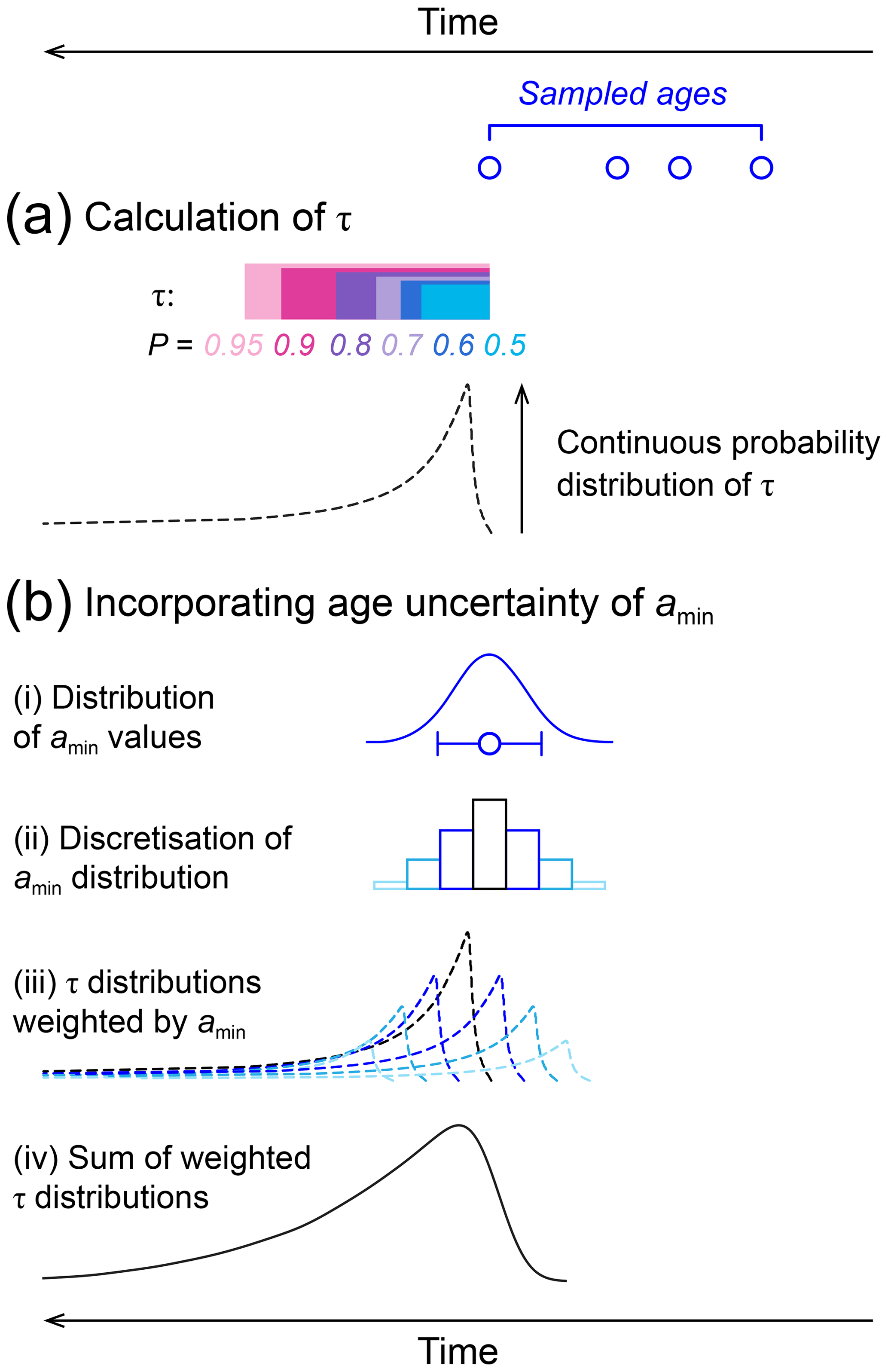
Figure 7Schematic demonstrating how to infer the timing of surface abandonment from a set of sampled ages. (a) Probable abandonment windows, τ, are calculated using Eq. (2) for discrete values of P (coloured bars). A continuous probability distribution of τ is equal to the density of P within each discrete increment of τ (dashed line); this can be generated using the MATLAB tool provided. (b) In reality, amin is not perfectly known and has an associated age uncertainty that must be accounted for. (i) The ±3σ uncertainty in amin provides a distribution of probable values of amin. (ii) The distribution of amin values is discretized. In the MATLAB tool, we have set this discretization to be one-tenth of the 1σ uncertainty in the youngest age, amin, to provide a highly resolved result (note that the illustration here shows much wider discretization bins for ease of visualization), but this discretization value can be modified. The discrete window of τ used to calculate the density of P is set to the same width. (iii) Probability distributions of τ are calculated for each potential value of amin (as per panel a), and weighted according to the probability distribution of amin values. (iv) The weighted, temporally shifted, τ distributions are then summed to produce a final probability distribution of surface abandonment timing that incorporates uncertainty into the youngest age.
However, real surface ages have associated uncertainties that must also be incorporated into the estimated abandonment ages (Fig. 7b). The MATLAB tool is designed to incorporate this uncertainty, and is explained in the following steps. First, we use ±3σ uncertainty in amin to characterize the probability distribution of potential amin values. In the example schematic (Fig. 7b) we assumed a normal distribution, as is typical for exposure ages of individual boulders, but alternative distributions could be used. This distribution of amin values is then discretized, and separate probability distributions of τ are calculated for each potential value of amin, i.e. repeating Fig. 7a. The resulting, temporally shifted probability distributions of τ are weighted according to the probability distribution of amin and summed, producing an overall probability distribution of likely abandonment ages that accounts for uncertainty in the youngest age (Fig. 7c). If the uncertainty in amin is small compared to τ calculated using Eq. (2), then incorporating age uncertainty will have little impact on the resulting probability distribution of abandonment ages. If the uncertainty on amin is large, it will have a greater influence on the final probability distribution of abandonment ages.
5.1 Implications for surface dating
Our artificial data provide new information about what measured ages represent when collected from aggraded surfaces that formed over non-negligible time spans. Crucially, our findings indicate that averages of sampled surface ages are likely to be imprecise representations of the mid-point of surface formation, which may not coincide with a particular external forcing event (Fig. 1). In contrast, surface abandonment typically occurs at a discrete moment in time and is more likely to coincide with external forcing events such as changes in climate or tectonics. By using artificial data, we have derived a set of probabilistic equations for inferring when a surface was likely to have been abandoned, based on a distribution of randomly sampled surface ages. These equations can complement and enhance interpretations based on any dataset comprising surface ages. The spreadsheet and the MATLAB tool allow for quantification of the full probability distribution of τ and the MATLAB tool additionally allows for the incorporation of uncertainty in the youngest age, amin.
While a distribution of ages is required for dating surfaces that have formed over extended periods of time, our analyses reveal that an increasing number of ages yield diminishing returns for constraining the timing of abandonment (Figs. 3d and 4) and the total duration of surface activity (Fig. 6). An appropriate number of surface ages will depend on the desired precision, but our results indicate that there is little to be gained by obtaining more than six to seven ages per surface (Figs. 3, 4, and 6), assuming no outliers, for the purposes of most geomorphological studies. To obtain substantially more information about a surface, an order of magnitude more ages would be required. As explained in Sect. 4.1, τ0 represents the maximum precision with which the abandonment age can, in principle, be inferred. For many natural surfaces, τ0 can range from a few centuries to ∼10 kyr (Fig. 5b), depending on the period of surface activity and the desired probability. Our methodology thus provides a new way to quantify how precisely a distribution of surface ages can be interpreted. This limit to precision should be considered in addition to the age uncertainty associated with cosmogenic nuclide exposure dating; both are important considerations when inverting landforms and sedimentary deposits for palaeo-environmental information (Foreman and Straub, 2017).
When sampling in the field, it may be advantageous to target different parts of an aggraded surface to capture as much of its period of activity as possible. This strategy applies to surfaces upon which the locus of deposition has systematically migrated during deposition. For example, if channel migration on an alluvial-fan surface resulted in a portion of its overall history being recorded in particular parts of the surface (e.g. Savi et al., 2016; Schürch et al., 2016; D'Arcy et al., 2017a, b), then greater spatial coverage would capture a greater range of ages. However, if each deposition event followed a random trajectory on the surface, resulting in all potentially selectable ages being spatially mixed, then it would be unnecessary to distribute sampling locations across the surface.
5.2 Case study: alluvial fans in the Laguna Salada Basin, Mexico
Here, we use a case study of alluvial-fan surfaces in the Laguna Salada Basin, Mexico, to demonstrate how our findings can be applied to real surfaces to gain new information about when they were abandoned.
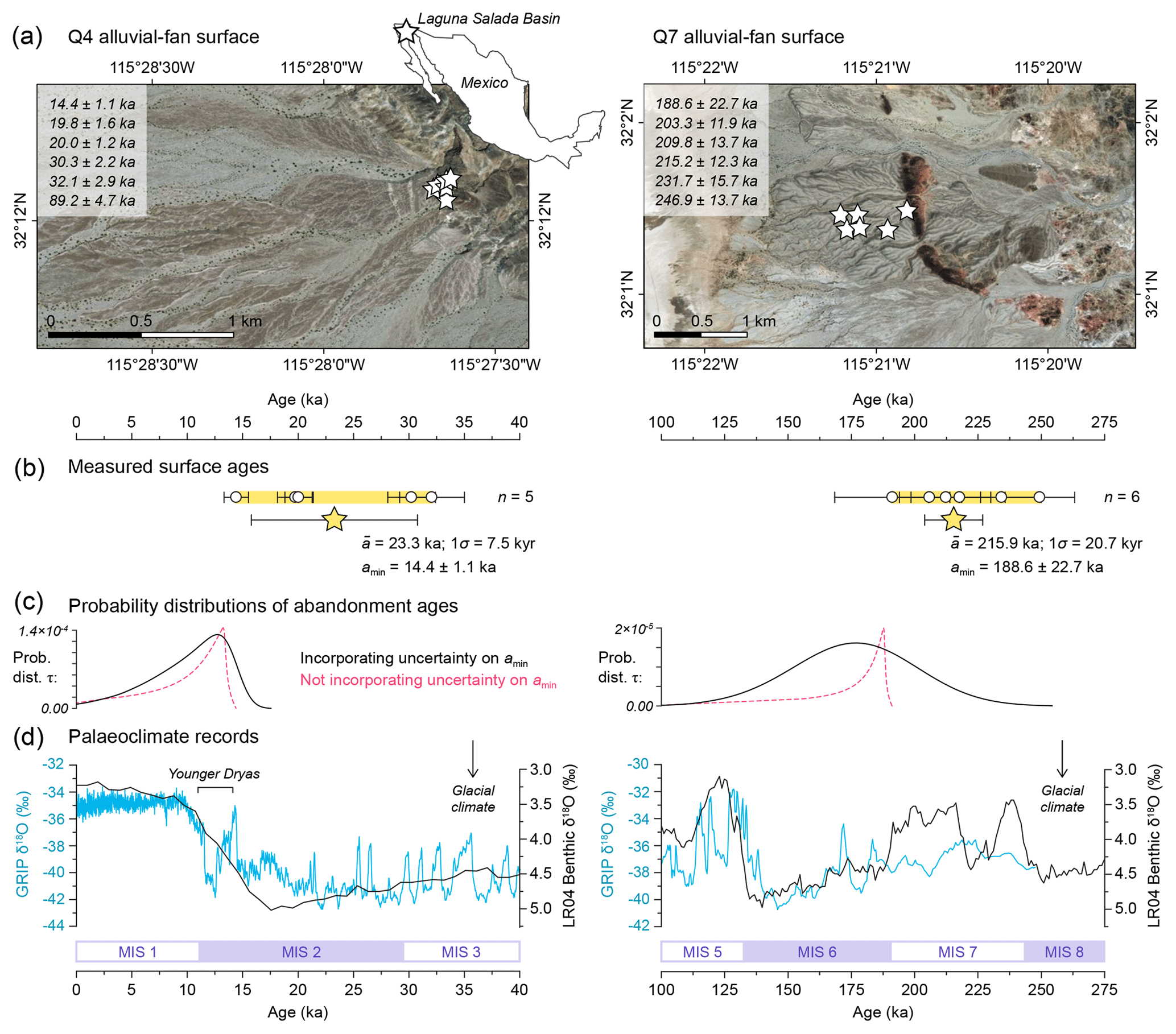
Figure 8Two alluvial-fan surfaces in the Laguna Salada Basin, northern Baja California, Mexico. Left column shows the Q4 surface and right column shows the Q7 surface, after Spelz et al. (2008). (a) Locations of surface boulders sampled for 10Be cosmogenic nuclide exposure dating. (b) Boulder exposure ages recalculated after Spelz et al. (2008) (white circles) and mean surface ages ±1σ (yellow stars). (c) Probability distributions of τ calculated using the MATLAB tool and incorporating uncertainty in amin (black). For illustrative purposes, probability distributions of τ are shown if uncertainty in amin is not incorporated (red dashed). (d) Selected palaeoclimate proxies: the GRIP ice core δ18O record from Greenland (blue; Johnsen et al., 1997) and the LR04 global benthic δ18O stack (black; Lisiecki and Raymo, 2005). Marine isotope stages (MIS) are indicated with boxes.
The Laguna Salada Basin is a half-graben in northern Baja California, Mexico. This basin contains well preserved alluvial fans eroded from the neighbouring Sierra El Mayor and Sierra de Los Cucapah, with at least eight generations of distinct fan surfaces formed by a sequence of aggradation and incision cycles. The ages of two of these fan surfaces – mapped as Q4 and Q7 – were estimated by Spelz et al. (2008) using 10Be exposure ages of stable surface boulders with no evidence of erosion or disturbance (Fig. 8). We used the CREp calculator (Martin et al., 2017) to update the exposure age estimates of Spelz et al. (2008) using the time-corrected Lal/Stone scaling scheme (Lal, 1991; Stone, 2000), the ERA40 atmosphere model (Uppala et al., 2005), the atmospheric 10Be-based virtual dipole moment (VDM) geomagnetic database of Muscheler et al. (2005) and Valet et al. (2005), and the current global reference sea level high latitude (SLHL) 10Be production rate of 4.13±0.20 g−1 yr−1 in the ICE-D database (Martin et al., 2017). We assume a sample density of 2.7 g cm−3 and no boulder erosion. The oldest age measured on the Q4 surface was excluded as an outlier by Spelz et al. (2008), and we maintain this interpretation. The remaining exposure ages span from 14.4±1.1 to 32.1±2.9 ka for Q4 (n=5) and 188.6±22.7 to 246.9±13.7 ka for Q7 (n=6) (Fig. 8b, yellow bars). On both fan surfaces, the dispersion of ages greatly exceeds the age uncertainty, suggesting that each surface was deposited over an extended period of time.
For both distributions of fan surface ages, we used Eqs. (2) through (6) to calculate probable abandonment windows, τ, for different values of P. For example, on the Q4 fan surface with an amin of 14.4±1.1 ka, τ= 3.3 kyr when P=0.5, suggesting a 50 % probability that the surface was abandoned within 3.3 kyr after amin, i.e. between 14.4 and 11.1 ka. The size of τ increases with P, as explained in Sect. 4.1, such that τ=12.0 kyr for the Q4 surface when P=0.95, i.e. the abandonment window ranges from 14.4 to 2.4 ka. The full probability distribution of τ is highly asymmetric (Fig. 8c, red dashed lines). Of course, the uncertainty in amin must also be accounted for. To do so, we used the MATLAB script with the required inputs – T and n; the desired number of iterations, amin; and the 1σ uncertainty in amin – to derive a continuous probability distribution of τ for each fan surface that incorporates age uncertainty (Fig. 8c, solid black lines). The probability distributions of τ incorporating age uncertainty, derived for both the Q4 and Q7 surfaces, illustrate how the likelihood of surface abandonment is distributed over time for two representative natural datasets. On the Q4 surface, the measured age uncertainty is small compared to τ, so the resulting τ distribution has an asymmetric shape that is primarily determined by the form of Eq. (2) and our artificial-data calibration (Figs. 3 and 4). The majority of the Q4 τ distribution occupies a short time span that is smaller than the spread of sampled surface ages; this result supports our reasoning that the timing of surface abandonment can, in some cases, be constrained more precisely than a representative age of surface formation (see Sect. 2). The age uncertainty in amin is significantly larger on the older Q7 surface and therefore dominates the probability distribution of τ, giving it a wider and more symmetrical shape despite the greater number of measured ages, n. This result underscores the importance of accounting for age uncertainty when using our equations to infer the likely timing of surface abandonment.
5.2.1 Climatic implications
Our estimates of when the Laguna Salada fans were abandoned have important climatic implications. Spelz et al. (2008) speculated that the aggradation and incision of the fan surfaces was partly controlled by past climate changes, and there is growing evidence that alluvial systems can be highly sensitive hydroclimate recorders (D'Arcy et al., 2017a, b; Terrizzano et al., 2017; Tofelde et al., 2017; Ratnayaka et al., 2018; Wickert and Schildgen, 2019). We explore this idea by comparing the surface age data with two palaeoclimate proxy records (Fig. 8d): the GRIP ice core δ18O record from Greenland (Johnsen et al., 1997) and the LR04 global benthic δ18O stack (Lisiecki and Raymo, 2005). These records primarily reflect the growth and decay of continental ice sheets, which are generalized into marine isotope stages (MIS).
The obtained Q7 ages clearly coincide with the broadly interglacial conditions of MIS 7, so we interpret that the surface was deposited throughout this stage. Our statistical analyses indicate that the Q7 surface was abandoned – in this case due to fan incision – during the subsequent MIS 6 and coinciding with a climatic transition to more glacial conditions. Indeed, 71 % of the area beneath the Q7 τ distribution falls within MIS 6 (191–130 ka), which we interpret as a 71 % likelihood that the surface was abandoned and incised during this stage. For the Q4 fan surface, the sampled ages alone indicate that abandonment coincided with the end of the Last Glacial Maximum (MIS 2) and the global shift to interglacial conditions in the Holocene. Spelz et al. (2008) interpreted this observation (fan incision during a shift to interglacial climate) to contradict the Q7 data (fan incision during a shift to more glacial conditions). However, supplementing the measured ages with our probabilistic analyses reveals that Q4 abandonment is likely to have occurred during the Younger Dryas, a short-lived climate episode from 12.9 to 11.7 ka during which the Northern Hemisphere climate returned to a cooler state (Carlson, 2013). We find that the peak of the τ distribution – i.e. the single most probable abandonment age – falls at 12.7 ka (Fig. 8c). This interpretation reconciles the Q7 and Q4 surfaces on the Laguna Salada fans, which would have both been incised as a result of climatic shifts towards more glacial conditions. This case study also demonstrates how our probabilistic approach, enabled by our use of artificial data, can be used to quantify the likelihood of individual abandonment scenarios and strengthen palaeoclimatic interpretations derived from alluvial deposits.
5.2.2 Tectonic and weathering implications
The results in Fig. 8 also have tectonic implications. The Laguna Salada fans are dissected by fault scarps related to the Laguna Salada fault and the Cañada David detachment; the largest Q7 scarp has an offset of 9.9 m (Spelz et al., 2008). Typically, studies divide the fault offset by the mean surface age (which for Q7 is 215.9 ka) to estimate a time-averaged slip rate, which would be 0.046 mm yr−1 in this example. However, as a scarp can only accumulate displacement once the surface has been abandoned, i.e. when it is no longer being resurfaced, the estimated age of abandonment may be a more appropriate timescale for determining a displacement rate. Accumulating a 9.9 m offset since 177 ka (the most likely abandonment age, Fig. 8c) would produce a time-averaged slip rate of 0.056 mm yr−1 an increase of 22 %. Following this logic, the probability distribution of τ could be translated into a probability distribution of time-averaged slip rates. For the Q4 fan surface, calculating a slip rate with a most likely abandonment age (e.g. 12.7 ka) instead of the mean surface age (23.3 ka) would result in an even larger increase in the calculated displacement rate of 83 %. Underestimating fault slip rates by this magnitude could have important implications for tectonic and fault hazard analyses.

Figure 9(a) Measured surface ages for the Laguna Salada alluvial-fan surfaces, following Fig. 8b. (b) Probability distributions of τ calculated using Eq. (2) and incorporating age uncertainty, where T is derived from the measured spread of surface ages using the mean case in Fig. 6 (black curves) and ±1σ uncertainties in T (red and blue curves).
Spelz et al. (2008) also measured the diffusional decay of fault scarp geometry over time, and used the calculated mean fan surface ages to derive time-integrated scarp mass diffusivities between ∼0.01 and 0.10 m2 kyr−1. Intriguingly, the authors interpreted these diffusivities to be anomalously low. More realistic values can be obtained by, again, using the estimated surface abandonment ages to calculate scarp mass diffusivity, rather than average surface ages. This approach would result in faster diffusion rates, as Spelz et al. (2008) expected, while recognizing that a fault scarp can only form and erode once a fan surface has been abandoned.
The alluvial fans of the Laguna Salada Basin provide a representative example of natural, aggraded geomorphic surfaces that are formed over a non-negligible period of activity and are dated with a small set of exposure ages that randomly sample the duration of surface activity. This case study demonstrates that our artificial-data approach can provide valuable constraints on the timing of surface abandonment based on a set of exposure ages, which can improve interpretations involving palaeoclimate, tectonics, and landform evolution.
5.3 Limitations to the probabilistic approach
Our artificial-data approach and the resulting parameterization of Eqs. (2) through (6) assume that a distribution of surface ages are obtained by randomly sampling the full duration of surface activity. In some cases, this assumption might be realistic. For example, the Q7 surface on the Laguna Salada fans (Fig. 8) was sampled in different places and produced ages spanning all of MIS 7, suggesting the full duration of surface activity might be well represented. If so, our approach could be symmetrically applied to the oldest sampled age to estimate the onset of deposition. In contrast, the Q4 surface was sampled entirely at the fan apex, where enhanced vertical aggradation makes it likely that the earliest deposits from this depositional episode have been buried. In practice, this sampling approach would improve estimates of when abandonment occurred. By clustering the surface ages towards the end of the depositional period, T would effectively shorten, given that our approach derives T empirically from the ages that are actually obtained from a surface, and τ would be constrained more precisely as a result. The total duration of deposition would be biased toward younger ages by the burial of older deposits, but this bias is unimportant when focusing on the timing of abandonment, which is a strength of our approach. However, vertical burial would mean that T (solved with Eq. 6) would no longer represent the total duration of deposition, and it would therefore be inappropriate to use our approach to estimate the onset of deposition.
Like burial, subsequent erosion of part of a surface might hide a fragment of the period of deposition from sampling. The implications of erosion depend on how spatially homogenous the surface is, i.e. whether erosion has randomly eliminated selectable ages from throughout the duration of activity or instead eradicated complete fragments of the time span of activity. Again, erosion would only impede our method of inferring the abandonment age if the youngest part of the duration of activity were destroyed. Given that burial and erosion are site specific, they cannot be universally incorporated into our equations and must be considered on an individual-case basis.
Our approach assumes that all sampled surface ages are true ages. In reality, incorrect ages are sometimes encountered when dating surfaces. For example, cosmogenic nuclide exposure ages may be biased towards older ages as a result of nuclide inheritance, as is interpreted to be the case with the oldest exposure age on the Laguna Salada Q4 fan surface (Fig. 8a). Including old outliers in our analyses would lead to an over-estimation of the size of both T and τ, and therefore unnecessarily imprecise estimates of the abandonment window, but would not change the position of amin. A more serious error would arise from incorrect young ages, e.g. resulting from erosion or shielding of boulders targeted for cosmogenic nuclide exposure dating. The inclusion of spurious young ages could expand the apparent period of surface activity T past the true timing of abandonment, leading to estimates of τ that are both too large and, more importantly, too young. Therefore, Eqs. (2)–(6) and the MATLAB tool should be applied to clean datasets that do not contain spurious ages, and particularly not spuriously young ages when attempting to calculate abandonment times.
Finally, our approach derives the true period of surface activity, T, from the measured age range amax−amin, based on the results of our artificial-data experiments (see Sect. 4.2 and Fig. 6). This step is necessary because the true duration of T is ultimately unknowable for natural surfaces, so we parameterize Eq. (6) using the mean ratio of among our artificial-data experiments. Of course, any given set of real surface ages might happen to capture a greater or smaller fraction of T than the mean case. For this reason, we also provide parameterizations of Eq. (6) for ±1 standard deviation (σ) above and below the mean ratio of , thus allowing ±1σ uncertainty in T to be tested. In practice, the uncertainty associated with T has little effect on the probability distributions of τ produced by Eq. (2), and so is likely to be insignificant for most geomorphological applications. To illustrate the sensitivity of τ to the uncertainty in T, we recalculate the probability distributions of τ for the Q4 and Q7 Laguna Salada alluvial-fan surfaces with the MATLAB tool (Fig. 9) using the ±1σ bounds on T (Fig. 6).
The uncertainty in T has a negligible effect on the probability distributions of τ for both the young and precisely dated Q4 surface where the τ distribution is most sensitive to the form of Eqs. (2) through (5), and the older, less precisely dated Q7 surface, where the τ distribution is most sensitive to the measured age uncertainty. This sensitivity analysis demonstrates how the conversion of amax−amin to T has little bearing on the estimated timings of surface abandonment. Nonetheless, our artificial-data calibration allows the ±1σ uncertainty in T to be calculated, if desired.
Our study uses artificial data to simulate depositional geomorphic surfaces that form over a non-negligible time span, and are subsequently dated with exposure ages on a set of randomly sampled boulders. We investigate scenarios that are representative of natural alluvial fans, which are commonly targeted for surface dating; however, our results may be more broadly applicable to other depositional landforms that form over protracted periods of time. Our findings suggest that, for a variety of different purposes, inferring the timing of surface abandonment may provide more informative and more precise interpretations than taking an average of measured surface ages. We use our artificial data to derive a set of probabilistic equations that can be applied to a distribution of real sampled surface ages to estimate a period of time within which abandonment is likely to have occurred with a given probability. These equations account for site-specific variables including the number of ages and the duration of activity for a particular surface and our artificial-data approach can be used to generate a probability distribution of likely abandonment ages. We provide a MATLAB script that generates a probability distribution of abandonment ages for a given surface and furthermore allows for the uncertainty associated with measured ages to be incorporated. The ability to constrain the timing of surface abandonment has useful applications for geomorphological studies that relate surface ages to tectonic deformation (e.g. deriving fault slip rates), climate (e.g. reconstructing past hydroclimate changes), or the rates of surface processes (e.g. weathering and landform evolution), a subset of which we demonstrate using a case study of alluvial-fan surfaces in the Laguna Salada Basin, Mexico. The statistical framework we introduce in this paper offers a new method of probabilistically estimating when a surface was abandoned, which can complement and enhance interpretations of any distribution of sampled ages obtained from surfaces that experienced a non-negligible period of deposition.
| amin | Youngest sampled age (kyr) |
| amax | Oldest sampled age (kyr) |
| Empirical constants relating k to P | |
| k | Exponential decay constant relating τ to n |
| Empirical constants relating τ0 to P and T | |
| n | Number of sampled ages |
| P | Probability (between 0 and 1) |
| Empirical constants for estimating T from amax and amin | |
| σ | Standard deviation |
| taban | Age of surface abandonment (kyr) |
| T | Time span of active surface formation (kyr) |
| τ | Abandonment window; the difference between amin and taban (kyr) |
| τ0 | Parameter relating τ to P and T (kyr) |
The MATLAB script used to analyse the data is provided in the Supplement.
All data in this article are presented in the main paper and are freely available online via the Figshare repository (D'Arcy et al., 2019); https://doi.org/10.6084/m9.figshare.8014583.
The supplement related to this article is available online at: https://doi.org/10.5194/esurf-7-755-2019-supplement.
MKD, JMT, and TFS conceived of the idea for this article. MKD performed the analyses and wrote the main text. TFS created the probabilistic sampling MATLAB script and contributed to interpretations. JMT contributed to the statistical analyses and PDN contributed to climatic interpretations. All authors commented on and contributed to the final article.
They authors declare that they have no conflict of interest.
We thank Luca Malatesta, an anonymous reviewer, and the associate editor Simon Mudd for constructive comments that improved the quality of the article.
Mitch K. D'Arcy was supported by an Alexander von Humboldt postdoctoral fellowship, a “Research Focus Earth Sciences” grant awarded by the University of Potsdam, and by the Emmy-Noether-Programm of the Deutsche Forschungsgemeinschaft, grant number SCHI 1241/1-1, awarded to Taylor F. Schildgen.
The article processing charges for this open-access
publication were covered by a Research
Centre of the Helmholtz Association.
This paper was edited by Simon Mudd and reviewed by Luca C. Malatesta and one anonymous referee.
Andrews, D. J. and Bucknam, R. C.: Fitting degradation of shoreline scarps by a nonlinear diffusion model, J. Geophys. Res.-Sol. Ea., 92, 12857–12867, https://doi.org/10.1029/JB092iB12p12857, 1987.
Brooke, S. A. S., Whittaker, A. C., Armitage, J. J., D'Arcy, M., and Watkins, S. E.: Quantifying sediment transport dynamics on alluvial fans from spatial and temporal changes in grain size, Death Valley, California, J. Geophys. Res.-Earth, 123, 2039–2067, https://doi.org/10.1029/2018JF004622, 2018.
Bufe, A., Burbank, D.W., Liu, L., Bookhagen, B., Qin, J., Chen, J., Li, T., Thompson Jobe, J. A., and Yang, H.: Variations of lateral bedrock erosion rates control planation of uplifting folds in the foreland of the Tian Shan, NW China, J. Geophys. Res.-Earth, 122, 2431–2467, https://doi.org/10.1002/2016JF004099, 2017.
Carlson, A. E.: The Younger Dryas climate event, Encyclopedia of Quaternary Science, 3, 126–134, https://doi.org/10.1016/B978-0-444-53643-3.00029-7, 2013.
Cesta, J. M. and Ward, D. J.: Timing and nature of alluvial fan development along the Chajnantor Plateau, northern Chile, Geomorphology, 273, 412–427, https://doi.org/10.1016/j.geomorph.2016.09.003, 2016.
Clow, T., Behr, W. M., and Helper, M. A.: Pleistocene to recent geomorphic and incision history of the northern Rio Grande gorge, New Mexico: Constraints from field mapping and cosmogenic 3He surface exposure dating, Geosphere, 15, 1–19, https://doi.org/10.1130/GES02017.1, 2019.
D'Arcy, M., Roda Boluda, D. C., Whittaker, A. C., and Carpineti, A.: Dating alluvial fan surfaces in Owens Valley, California, using weathering fractures in boulders, Earth Surf. Proc. Land., 40, 487–501, https://doi.org/10.1002/esp.3649, 2015.
D'Arcy, M., Whittaker, A. C., and Roda-Boluda, D. C.: Measuring alluvial fan sensitivity to past climate changes using a self-similarity approach to grain-size fining, Death Valley, California, Sedimentology, 64, 388–424, https://doi.org/10.1111/sed.12308, 2017a.
D'Arcy, M., Roda-Boluda, D. C., and Whittaker, A. C.: Glacial-interglacial climate changes recorded by debris flow fan deposits, Owens Valley, California, Quaternary Sci. Rev., 169, 288–311, https://doi.org/10.1016/j.quascirev.2017.06.002, 2017b.
D'Arcy, M., Mason, P. J., Roda-Boluda, D. C., Whittaker, A. C., Lewis, J. M. T., and Najorka, J.: Alluvial fan surface ages recorded by Landsat-8 imagery in Owens Valley, California, Remote Sens. Environ., 216, 401–414, https://doi.org/10.1016/j.rse.2018.07.013, 2018.
D'Arcy, M., Schildgen, T. F., Turowski, J. M., and DiNezio, P.: Artificial data – Probabilistic age sampling, Figshare data repository, https://doi.org/10.6084/m9.figshare.8014583, 2019.
Denn, A. R., Bierman, P. R., Zimmerman, S. R. H., Caffee, M. W., Corbett, L. B., and Kirby, E.: Cosmogenic nuclides indicate that boulder fields are dynamics, ancient, multigenerational features, GSA Today, 28, 4–10, https://doi.org/10.1130/GSATG340A.1, 2017.
Dühnforth, M., Densmore, A. L., Ivy-Ochs, S., Allen, P. A., and Kubik, P. W.: Timing and patterns of debris flow deposition on Shepherd and Symmes creek fans, Owens Valley, California, deduced from cosmogenic 10Be, J. Geophys. Res., 112, F03S15, https://doi.org/10.1029/2006JF000562, 2007.
Finnegan, N. J., Schumer, R., and Finnegan, S.: A signature of transience in bedrock river incision rates over timescales of 104–107 years, Nature, 505, 391–394, https://doi.org/10.1038/nature12913, 2014.
Frankel, K. L., Brantley, K. S., Dolan, J. F., Finkel, R. C., Klinger, R. E., Knott, J. R., Machette, M. N., Owen, L. A., Phillips, F. M., Slate, J. L., and Wernicke, B. P.: Cosmogenic 10Be and 36Cl geochronology of offset alluvial fans along the northern Death Valley fault zone: Implications for transient strain in the eastern California shear zone, J. Geophys. Res., 112, B06407, https://doi.org/10.1029/2006JB004350, 2007.
Foreman, B. Z. and Straub, K. M.: Autogenic geomorphic processes determine the resolution and fidelity of terrestrial paleoclimate records, Sci. Adv., 3, 1–11, https://doi.org/10.1126/sciadv.1700683, 2017.
Frankel, K. L., Dolan, J. F., Owen, L. A., Ganev, P., and Finkel, R. C.: Spatial and temporal constancy of seismic strain release along an evolving segment of the Pacific–North America plate boundary, Earth Planet. Sc. Lett., 304, 565–576, https://doi.org/10.1016/j.epsl.2011.02.034, 2011.
Foster, M. A., Anderson, R. S., Gray, H. J., and Mahan, S. A.: Dating of river terraces along Lefthand Creek, western High Plains, Colorado, reveals punctuated incision, Geomorphology, 295, 176–190, https://doi.org/10.1016/j.geomorph.2017.04.044, 2017.
Ganev, P. N., Dolan, J. F., Frankel, K. L., and Finkel, R. C.: Rates of extension along the Fish Lake Valley fault and transtensional deformation in the Eastern California shear zone–Walker Lane belt, Lithosphere, 2, 33–49, https://doi.org/10.1130/L51.1, 2010.
Gosse, J. C.: Terrestrial Cosmogenic Nuclide Techniques for Assessing Exposure History of Surfaces and Sediments in Active Tectonic Regions, in: Tectonics of Sedimentary Basins: Recent Advances, edited by: Busby, C. and Azor, A., Blackwell Publishing Ltd, Chichester, UK, 63–79, 2011.
Hanks, T. C., Bucknam, R. C., Lajoie, K. R., and Wallace, R. E.: Modification of wave-cut and faulting-controlled landforms, J. Geophys. Res.-Sol. Ea., 89, 5771–5790, https://doi.org/10.1029/JB089iB07p05771, 1984.
Hughes, A., Rood, D. H., Whittaker, A. C., Bell, R. E., Rockwell, T. K., Levy, Y., Wilcken, K. M., Corbett, L. B., Bierman, P. R., DeVecchio, D. E., Marshall, S. T., Gurrola, L. D., and Nicholson, C.: Geomorphic evidence for the geometry and slip rate of a young, low-angle thrust fault: Implications for hazard assessment and fault interaction in complex tectonic environments, Earth Planet. Sc. Lett., 504, 198–210, https://doi.org/10.1016/j.epsl.2018.10.003, 2018.
Johnsen, S. J., Clausen, H. B., Dansgaard, W., Gundestrup, N. S., Hammer, C. U., Andersen, U., Andersen, K. K., Hvidberg, C. S., Dahl-Jensen, D., Steffensen, J. P., and Shoji, H.: The δ18O record along the Greenland Ice Core Project deep ice core and the problem of possible Eemian climatic instability, J. Geophys. Res.-Oceans, 102, 26397–26410, https://doi.org/10.1029/97JC00167, 1997.
Lal, D.: Cosmic ray labeling of erosion surfaces: In situ nuclide production rates and erosion models, Earth Planet. Sc. Lett., 104, 424–439, https://doi.org/10.1016/0012-821X(91)90220-C, 1991.
Lisiecki, L. E. and Raymo, M. E.: A Pliocene-Pleistocene stack of 57 globally distributed benthic δ18O records, Paleoceanography, 20, PA1003, https://doi.org/10.1029/2004PA001071, 2005.
Macklin, M. G., Fuller, I. C., Lewin, J., Maas, G. S., Passmore, D. G., Rose, J., Woodward, J. C., Black, S., Hamlin, R. H. B., and Rowan, J. S.: Correlation of fluvial sequences in the Mediterranean basin over the last 200 ka and their relationship to climate change, Quaternary Sci. Rev., 21, 1633–1641, https://doi.org/10.1016/S0277-3791(01)00147-0, 2002.
Malatesta, L. C., Prancevic, J. P., and Avouac, J.-P.: Autogenic entrenchment patterns and terraces due to coupling with lateral erosion in incising alluvial channels, J. Geophys. Res.-Earth, 122, 335–355, https://doi.org/10.1002/2015JF003797, 2017.
Martin, L. C. P., Blard, P.-H., Balco, G., Lavé, J., Delunel, R., Lifton, N., and Laurent, V.: The CREp program and the ICE-D production rate calibration database: A fully parameterizable and updated online tool to compute cosmic-ray exposure ages, Quat. Geochronol., 38, 25–49, https://doi.org/10.1016/j.quageo.2016.11.006, 2017.
Mouslopoulou, V., Begg, J., Fülling, A., Moraetis, D., Partsinevelos, P., and Oncken, O.: Distinct phases of eustatic and tectonic forcing for late Quaternary landscape evolution in southwest Crete, Greece, Earth Surf. Dynam., 5, 511–527, https://doi.org/10.5194/esurf-5-511-2017, 2017.
Muscheler, R., Beer, J., Kubik, P. W., and Synal, H.-A.: Geomagnetic field intensity during the last 60,000 years based on 10Be and 36Cl from the Summit ice cores and 14C, Quaternary Sci. Rev., 24, 1849–1860, https://doi.org/10.1016/j.quascirev.2005.01.012, 2005.
Owen, L. A., Frankel, K. L., Knott, J. R., Reynhout, S., Finkel, R. C., Dolan, J. F., and Lee, J.: Beryllium-10 terrestrial cosmogenic nuclide surface exposure dating of Quaternary landforms in Death Valley, Geomorphology, 125, 541–557, https://doi.org/10.1016/j.geomorph.2010.10.024, 2011.
Owen, L. A., Clemmens, S. J., Finkel, R. J., and Gray, H.: Late Quaternary alluvial fans at the eastern end of the San Bernardino Mountains, Southern California, Quaternary Sci. Rev., 87, 114–134, https://doi.org/10.1016/j.quascirev.2014.01.003, 2014.
Ratnayaka, K., Hetzel, R., Hornung, J., Hampel, A., Hinderer, M., and Frechen, M.: Postglacial alluvial fan dynamics in the Cordillera Oriental, Peru, and palaeoclimatic implications, Quaternary Res., 91, 431–449, https://doi.org/10.1017/qua.2018.106, 2018.
Regmi, N. R., McDonald, E. V., and Bacon, S. N.: Mapping Quaternary alluvial fans in the southwestern United States based on multiparameter surface roughness of lidar topographic data, J. Geophys. Res.-Earth, 119, 12–27, https://doi.org/10.1002/2012JF002711, 2014.
Sarıkaya, M. A., Yıldırım, C., and Çiner, A.: Late Quaternary alluvial fans of Emli Valley in the Ecemiş Fault Zone, south central Turkey: Insights from cosmogenic nuclides, Geomorphology, 228, 512–525, https://doi.org/10.1016/j.geomorph.2014.10.008, 2015.
Savi, S., Schildgen, T. F., Tofelde, S., Wittmann, H., Scherler, D., Mey, J., Alonso, R. N., and Strecker, M. R.: Climatic controls on debris-flow activity and sediment aggradation: The Del Medio fan, NW Argentina, J. Geophys. Res.-Earth, 121, 2424–2445, https://doi.org/10.1002/2016JF003912, 2016.
Schildgen, T. F., Cosentino, D., Bookhagen, B., Niedermann, S., Yıldırım, C., Echtler, H., Wittmann, H., and Strecker, M. R.: Multi-phased uplift of the southern margin of the Central Anatolian plateau, Turkey: A record of tectonic and upper mantle processes, Earth Planet. Sc. Lett., 317–318, 85–95, https://doi.org/10.1016/j.epsl.2011.12.003, 2012.
Schildgen, T. F., Robinson, R. A. J., Savi, S., Phillips, W. M., Spencer, J. Q. G., Bookhagen, B., Scherler, D., Tofelde, S., Alonso, R. N., Kubik, P. W., Binnie, S. A., and Strecker, M. R.: Landscape response to late Pleistocene climate change in NW Argentina: Sediment flux modulated by basin geometry and connectivity, J. Geophys. Res.-Earth, 121, 392–414, https://doi.org/10.1002/2015JF003607, 2016.
Schürch, P., Densmore, A. L., Ivy-Ochs, S., Rosser, N. J., Kober, F., Schlunegger, F., McArdell, B., and Alfimov, V.: Quantitative reconstruction of late Holocene surface evolution on an alpine debris-flow fan, Geomorphology, 275, 46–57, https://doi.org/10.1016/j.geomorph.2016.09.020, 2016.
Simpson, G. and Castelltort, S.: Model shows that rivers transmit high-frequency climate cycles to the sedimentary record, Geology, 40, 1131–1134, https://doi.org/10.1130/G33451.1, 2012.
Spelz, R. M., Fletcher, J. M., Owen, L. A., and Caffee, M. W.: Quaternary alluvial-fan development, climate and morphologic dating of fault scarps in Laguna Salada, Baja California, Mexico, Geomorphology, 102, 578–594, https://doi.org/10.1016/j.geomorph.2008.06.001, 2008.
Steffen, D., Schlunegger, F., and Preusser, F. Drainage basin response to climate change in the Pisco valley, Peru, Geology, 37, 491–494, https://doi.org/10.1130/G25475A.1, 2009.
Stone, J. O.: Air pressure and cosmogenic isotope production, J. Geophys. Res., 105, 23753–23759, https://doi.org/10.1029/2000JB900181, 2000.
Terrizzano, C. M., García Morabito, E., Christl, M., Likerman, J., Tobal, J., Yamin, M., and Zech, R.: Climatic and tectonic forcing on alluvial fans in the southern Central Andes, Quaternary Sci. Rev., 172, 131–141, https://doi.org/10.1016/j.quascirev.2017.08.002, 2017.
Tofelde, S., Schildgen, T. F., Savi, S., Pingel, H., Wickert, A. D., Bookhagen, B., Wittmann, H., Alonso, R. N., Cottle, J., and Strecker, M. R.: 100 kyr fluvial cut-and-fill terrace cycles since the Middle Pleistocene in the southern Central Andes, NW Argentina, Earth Planet. Sc. Lett., 473, 141–153, https://doi.org/10.1016/j.epsl.2017.06.001, 2017.
Uppala, S. M., Kållberg, P. W., Simmons, A. J., Andrae, U., Bechtold, V. D. C., Fiorino, M., Gibson, J. K., Haseler, J., Hernandez, A., Kelly, G. A., and Li, X.:The ERA-40 re-analysis, Q. J. Roy. Meteor. Soc., 131, 2961–3012, https://doi.org/10.1256/qj.04.176, 2005.
Valet, J.-P., Meynadier, L., and Guyodo, Y. Geomagnetic dipole strength and reversal rate over the past two million years, Nature, 435, 802–805, https://doi.org/10.1038/nature03674, 2005.
White, A. F., Blum, A. E., Schulz, M. S., Bullen, T. D., Harden, J. W., and Peterson, M. L.: Chemical weathering rates of a soil chronosequence on granitic alluvium: I. Quantification of mineralogical and surface area changes and calculation of primary silicate reaction rates, Geochim. Cosmochim. Ac., 60, 2533–2550, https://doi.org/10.1016/0016-7037(96)00106-8, 1996.
White, A. F., Schulz, M. S., Vivit, D.V., Blum, A. E., Stonestrom, D. A., and Harden, J. W.: Chemical weathering rates of a soil chronosequence on granitic alluvium: III. Hydrochemical evolution and contemporary solute fluxes and rates, Geochim. Cosmochim. Ac., 69, 1975–1996, https://doi.org/10.1016/j.gca.2004.10.003, 2005.
Wickert, A. D. and Schildgen, T. F.: Long-profile evolution of transport-limited gravel-bed rivers, Earth Surf. Dynam., 7, 17–43, https://doi.org/10.5194/esurf-7-17-2019, 2019.