2.1 Experimental setup

The sensitivity of catchment hydro-morphological response to changes in the spatial properties of rainfall during heavy rainfall events was examined using a combination of models. The numerical experiment is composed of two steps: (i) generation of an ensemble of space-time rainfall fields under scenarios of temperature change, and (ii) simulation of hydro-morphological response in runoff and sediment yield with this ensemble.

First, a time series of mean areal rainfall over the domain is simulated. The time series follows a temporal structure of a design storm characterized by a Gaussian shape that is assumed representative of a heavy rainfall event for present climate conditions (Fig. 2). A rainfall generator model (Sect. 2.2) is then used to generate multiple realizations of gridded rainfall for the design storm. In practice, the rainfall generator downscales the areal rainfall over the domain to a finer spatial resolution. Each of the realizations has a different 2-dimensional representation of the rainfall intensities in space. In this way, the spatial rainfall variability (stochasticity) is explicitly accounted for (see further discussion on the role of stochastic rainfall spatial variability by Paschalis et al., 2014; Peleg et al., 2017a, 2018b, 2019). The model was set to simulate two types of rainfall: stratiform and convective, with associated values of peak rainfall intensities and spatial variability in rainfall intensity (see Sect. 3.2).

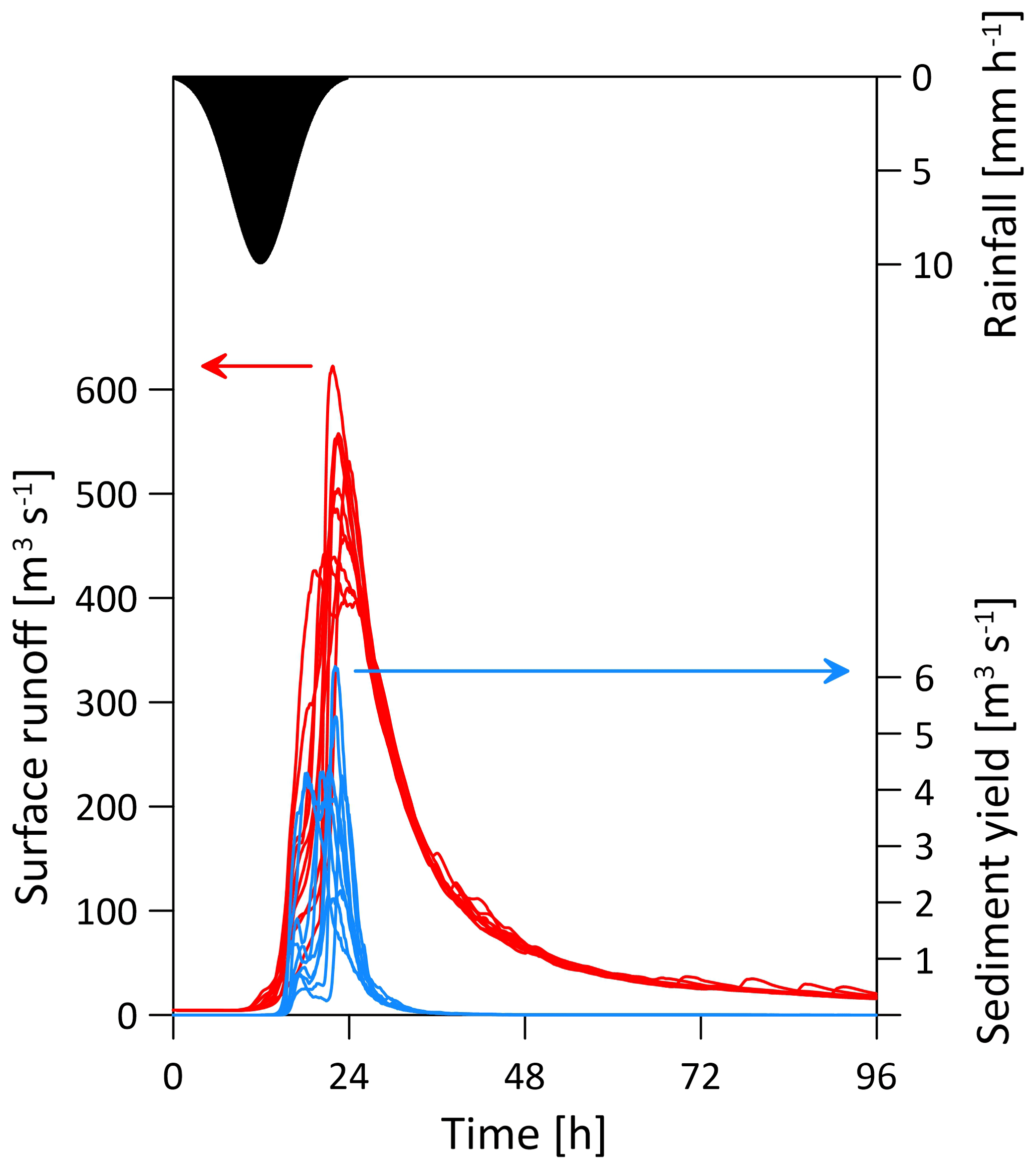
Figure 2Illustration of the mean rainfall intensity over the catchment area for the design storm (black area) and the respectively generated stream runoff (red lines) and sediment yields (blue lines) from 10 stochastic rainfall realizations produced with the rainfall generator model.

Download

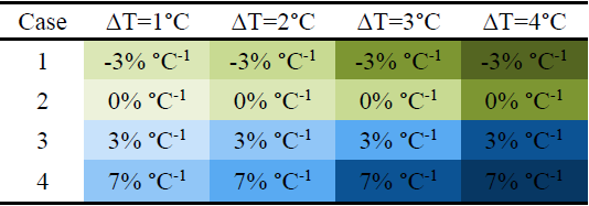
The rainfall fields are then modified using the rainfall generator to follow four “temperature increase scenarios” and four “areal rainfall scenarios” for convective and stratiform types (16×2 spatial scenarios altogether, see Table 1). In all of the scenarios, the peak rainfall intensity at the grid scale (i.e. the grid cells with the maximum rainfall intensities at the time the areal rainfall peaks) is assumed to intensify at a rate of 7 % ^∘C⁻¹, which corresponds to the CC rate (Trenberth et al., 2003) and is representative of a fully saturated air column. The areal rainfall scenarios refer to four possible cases: (case 1) a decrease in the mean areal rainfall (by −3 % ^∘C⁻¹) that is associated with a decrease in the area of heavy rainfall (defined as the total area above a rain intensity threshold of 10 mm h⁻¹), (case 2) no change in the mean areal rainfall (0 % ^∘C⁻¹) but a small decrease in the area of heavy rainfall, (case 3) an increase in the mean areal rainfall (by 3 % ^∘C⁻¹) with a small increase in the area of heavy rainfall, and (case 4) an increase in the mean areal rainfall of the same rate as peak rainfall (7 % ^∘C⁻¹) with a significant increase in the area of heavy rainfall (Table 1 and Fig. 1).

Peak rainfall intensity can intensify at a higher rate than 7 % ^∘C⁻¹, potentially increasing the consequences for the fluvial response. To further demonstrate this point, a subset of the numerical experiments (case 2 and only for the convective rainfall type) was extended to include intensification of the peak rainfall at the grid scale from the CC rate (7 % ^∘C⁻¹) to a super-CC rate (14 % ^∘C⁻¹; e.g. Lenderink and Van Meijgaard, 2008, 2CC from hereafter).

Table 1The four “temperature increase scenarios” (ΔT), and the four scenarios for changes in the mean areal rainfall intensity (expressed by % ^∘C⁻¹). The scenarios apply for both stratiform and convective types, with different peak intensities and spatial statistical properties of rainfall. Colours represent qualitatively changes in the area of the intense rainfall, from a large increase (dark blue) to a large decrease (dark green). For all the scenarios, the peak rainfall intensity is assumed to increase at a rate of 7 % ^∘C⁻¹.

Download Print Version

An example of simulated rainfall fields for the four spatial rainfall scenarios, for the case with a temperature increase of 3 ^∘C, is presented in Fig. 3. The effects of the changes in the spatial structure of the rainfall on the spatial correlation of the field are shown in Fig. 4.

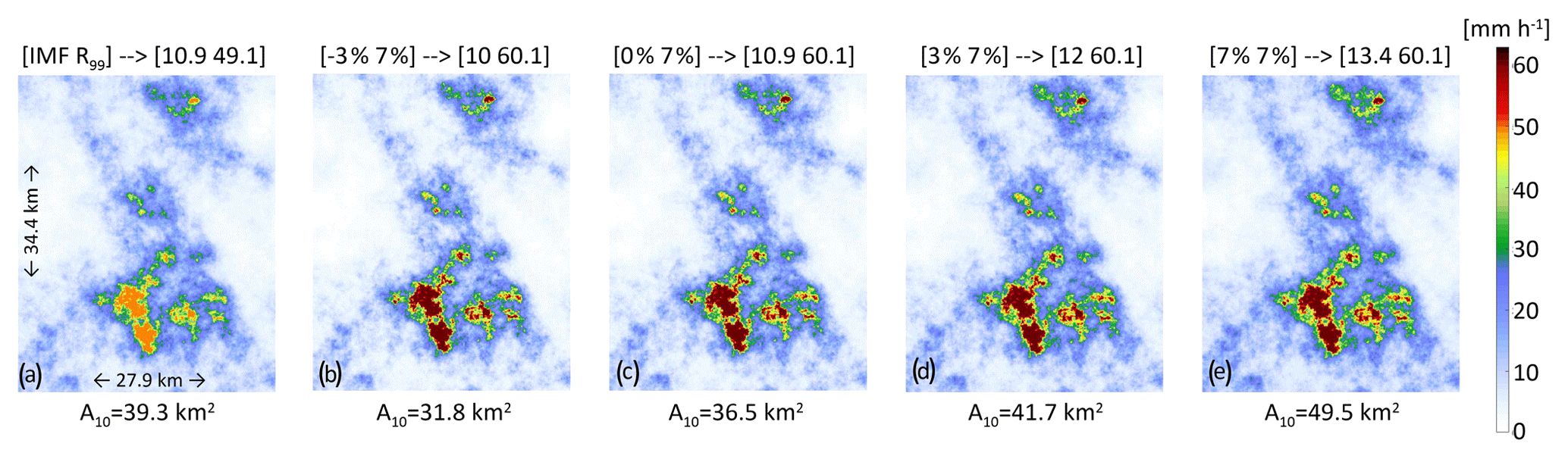
Figure 3(a) An example of a stratiform simulated rainfall field for a given time step. (b–e) Plots of the rainfall field with four different “areal rainfall scenarios” (Table 1) and for a specific “temperature scenario” of ΔT=3 ^∘C. IMF refers to changes in the mean areal rainfall (% ^∘C⁻¹) and R₉₉ refers to changes in the peak rainfall intensity (% ^∘C⁻¹) in comparison to (a); the absolute values of mean areal rainfall and peak rainfall intensity are given in parentheses (mm h⁻¹). A₁₀ refers to the total area (km²) above a rain intensity threshold of 10 mm h⁻¹.

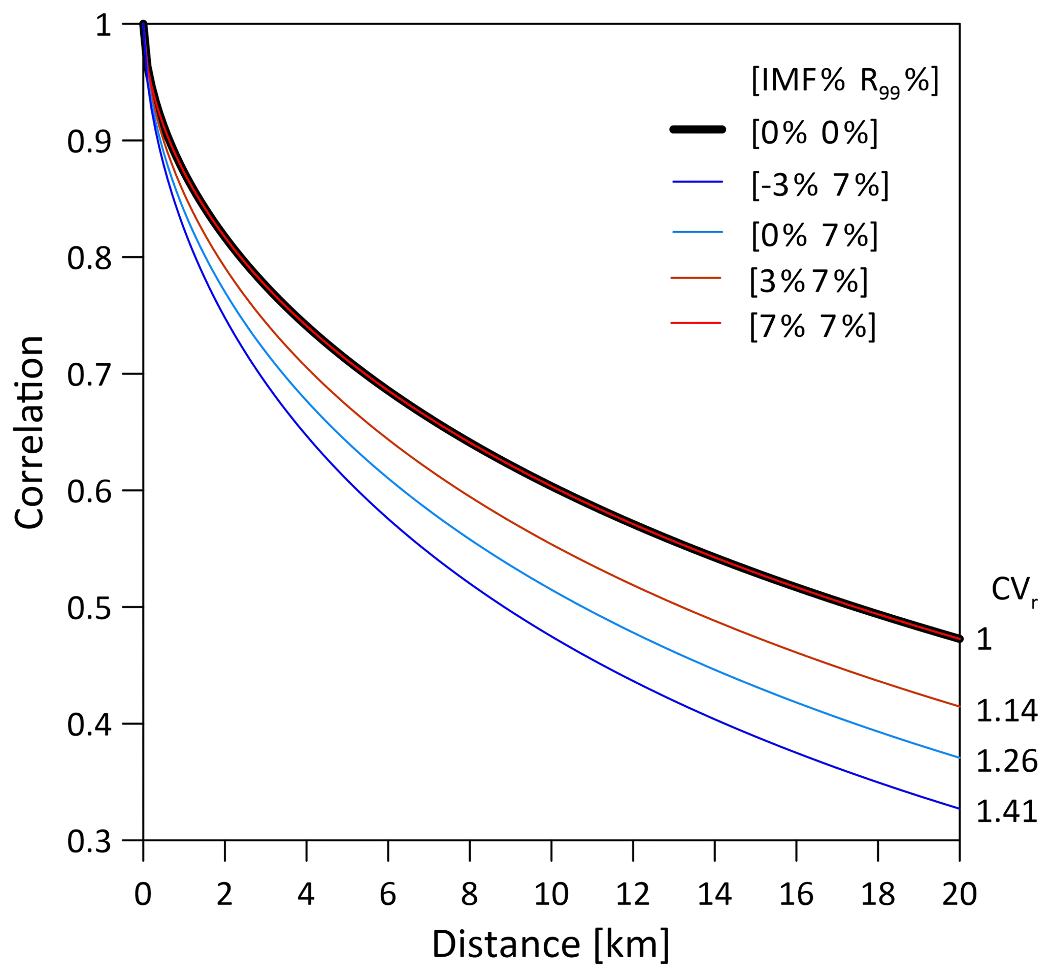
Figure 4Spatial correlation of the rainfall fields that are presented in Fig. 3 for the specific case of ΔT=3 ^∘C. The correlation is computed on the spectral densities of the fields following Peleg et al. (2019) and for each case the spatial coefficient of variation of the field CV_r is given. IMF refers to changes in the mean areal rainfall (% ^∘C⁻¹) and R₉₉ refers to changes in the peak rainfall intensity (% ^∘C⁻¹).

Download

In the second stage, the multiple stochastic realizations of design storms that were simulated for each of the 16 different scenarios and for the 2CC experiment were fed into a landscape evolution model (Sect. 2.3) to simulate the hydro-morphological response, i.e. streamflow and sediment transport (Fig. 2). The sensitivity of the response to the changes in rainfall spatial properties was finally analysed.

2.2 Space-time stochastic rainfall generator model

Gridded stochastic rainfall generator models can be used to generate multiple realizations of a given (design) storm (McRobie et al., 2013; Paschalis et al., 2014; Peleg et al., 2018b; Shah et al., 1996a, b). The realizations preserve the temporal evolution of the mean areal rainfall over the domain, but they differ in how the rainfall intensities are distributed in space within the domain. Here a simplified version of the STREAP (Space-Time Realizations of Areal Precipitation) rainfall generator model was used for generating high-resolution space-time rainfall fields (Paschalis et al., 2013). STREAP is based on previous space-time rainfall generators (Bell, 1987; Kundu and Bell, 2003; Pegram and Clothier, 2001a, b) and was recently further developed by Peleg et al. (2017b). The model simulates rainfall fields in three steps: (i) the length of the storms and the intra-storm periods are generated, (ii) the temporal evolution of the mean areal intensity over the domain and the fraction of wet area are simulated, and (iii) these time series are translated into intermittent space-time rainfall fields. As the design storm used in this study is predefined, only step (iii) is required in this study. Several modifications to this step were required in order to tailor the spatial structure of the rainfall fields to follow prescribed changes in both the peak and areal rainfall with temperature. The STREAP model is discussed in detail by Paschalis et al. (2013) and here only a brief description of step (iii) and specific modifications used in this case study are presented.

The intermittent rainfall field is simulated as a probability transformation of an isotropic Gaussian random field that is computed using the fast Fourier transform method. As in previous studies, we assume that rainfall intensity is spatially distributed following a log-normal distribution (e.g. Paschalis et al., 2013, 2014; Peleg et al., 2017b, 2018b, 2019). A log-normal function is therefore applied to convert the isotropic Gaussian field to the intermittent rainfall field. The information needed for this transformation is the mean areal rainfall over the domain (abbreviated hereafter as IMF, following the notations of Pegram and Clothier, 2001a) and the rainfall coefficient of variation (CV_r) in space, which is a model parameter. Assuming that the rainfall covers the entire domain (i.e. the wet area ratio WAR is equal to 1), the intermittent rainfall fields are expressed as the following (see Paschalis et al., 2013 for details):

where $R(x,y,t)$ is the rainfall intensity in space and time, LN⁻¹ is the inverse cumulative log-normal distribution, and $U\left[G\right(x,y,t\left)\right]$ represents the percentiles in space and time of the latent isotropic Gaussian field. The parameters of the log-normal distribution, μ_r and σ_r, are expressed as

and

The peak rainfall intensity at the grid scale is defined as the inverse log-normal of the 99th percentile, notated as R₉₉ and expressed as

Equation (4) can be simplified to find a unique relation between the mean areal rainfall intensity (IMF) and the peak rainfall intensity at each time step:

The rainfall spatial coefficient of variation is a model parameter that changes depending on the scenarios. If, for example, the CV_r value for the reference simulation (i.e. ΔT=0 ^∘C) is equal to 1, the CV_r values will increase with an increasing difference between the scaling of the peak rainfall intensity and the areal rainfall. Convective and stratiform rainfall types have different reference values of CVr. An example of how CV_r changes as a function of the scaling of the peak rainfall and the areal rainfall intensities is presented in Fig. 4.

2.3 Hydro-morphological model

The hydrological and geomorphic response to rainfall is explored using a landscape evolution model (LEM; see review paper by Tucker and Hancock, 2010). The CAESAR (Coulthard et al., 2002) and CAESAR-Lisflood models (Coulthard et al., 2013) are grid-based LEMs that have been widely used to simulate morphodynamic changes from short temporal (< 1 year or event based) and small spatial (< 1 km²) scales (Coulthard et al., 2012a; Hoober et al., 2017) to long temporal (> 10⁴ year) and large spatial (10³ km²) scales (Coulthard and Van De Wiel, 2017; Hancock et al., 2010, 2015). Both models were used in the past to explore hydro-morphologic sensitivity to climate change and rainfall temporal variability (Coulthard et al., 2012b; Hancock, 2009, 2012; Hancock and Coulthard, 2012; Hoober et al., 2017). Recent versions of the CAESAR-Lisflood model have the ability to use gridded rainfall as an input (Coulthard and Skinner, 2016; Skinner et al., 2020), which is an essential ability for this study. This feature is lacking in many other LEMs. Surface runoff in the model is computed using the TOPMODEL hydrological model (Beven and Kirkby, 1979) and is routed downstream using the LISFLOOD-FP model (Bates et al., 2010), which generates flow depths and velocities. Fluvial erosion can be simulated using either Wilcock and Crowe, Einstein, or Meyer-Peter–Muller equations, moving sediment that is stored in an active-layer system that can handle up to nine grain sizes. Lateral erosion, slope processes, soil development, and interaction with vegetation are also simulated by the model. Version “1.9h” of the model was used in this study, and no modifications were made to the source code. For further details on the model, the reader is referred to Coulthard et al. (2013).

3.1 Data

We set the numerical models to simulate the impacts of a heavy rainfall event that is similar to the event that occurred in August 2005 (data for the period between 14 and 28 August were used). Rainfall data were gathered from the Swiss Federal Office for Meteorology and Climatology (MeteoSwiss) from two different products. Rainfall records at 10 min temporal resolution were obtained from three MeteoSwiss – SwissMetNet – ground stations surrounding the catchment (Fig. 5). Mean areal rainfall over the domain at 10 min was computed by averaging rainfall from the three locations. It was then temporally downscaled to 5 min resolution using linear interpolation. We assume that by using the data from these three stations, the temporal dynamics of the mean areal rainfall over the catchment is adequately represented (i.e. the timing of the storm is preserved). However, the mean areal rainfall intensities might not be representative for the entire catchment as the three meteorological stations are located in the northern part of the catchment (Fig. 5). Therefore, the rainfall amounts were corrected using data from gridded 1 km daily rainfall estimates that were derived from the MeteoSwiss product RhiresD (MeteoSwiss, 2016; Schwarb, 2000) that covers the entire catchment. For each day, the mean areal rainfall over the catchment was computed from the RhiresD product. The 5 min rainfall intensities were aggregated to the daily scale, compared with the daily RhiresD estimates, and corrected using a multiplicative factor. The final time series of the mean areal rainfall for the observed storm in August 2005 is presented in Fig. 6.

Figure 6Illustration of the heavy rainfall event of August 2005 in the Kleine Emme catchment. The black line represents the mean areal rainfall over the catchment. The blue and red lines represent the observed and simulated hydrographs, respectively, at the outlet of the catchment. The 10 simulated lines are a result of the stochastic downscaling of the areal rainfall to a finer (100 m) spatial resolution using the rainfall generator model and its range represents the sensitivity of the hydrological response to the spatial rainfall variability.

Download

Hourly streamflow data were supplied by the Swiss Federal Office for the Environment for the Emmen station located at the outlet of the catchment (Fig. 5). Estimates of the sediment yield, grain size distribution, and the geomorphologic response to heavy rainfall events for the Kleine Emme, and for nearby catchments that are representative of the study area, were obtained from multiple sources (Bezzola and Hegg, 2008; Heimann et al., 2015; Rickenmann et al., 2008, 2016; Rickenmann and Koschni, 2010; Rickenmann and McArdell, 2007; Steeb et al., 2017). The digital elevation map (Fig. 5) and bedrock map (Supplement Fig. S1) were supplied by the Swiss Federal Office of Topography at 25 m resolution and were upscaled to 100 m resolution, which was the resolution used for model simulations. The surface roughness map (Fig. S2) at 100 m resolution was prepared based on a land use map that was obtained from the Swiss Federal Statistical Office following the classification suggested by Te Chow (1959).

3.2 Setup of the rainfall generator model

The parameters of the rainfall generator model (Table 2) were not calibrated to reproduce the statistics of a specific heavy rainfall event that was observed over the catchment but to simulate realistic space-time structure of rainfall fields over the Alpine region. The rainfall fields are simulated to move with a constant speed and direction as the hydrological response is sensitive to these parameters (Paschalis et al., 2014; Yakir and Morin, 2011). The parameters for the correlation length and storm velocity and direction follow reference values that were found by analysing rainfall fields obtained from a weather radar system in nearby Alpine catchments (Peleg et al., 2017a, b, 2019). The CV_r parameter was set to be equal to 1 for the simulations of the real storm and for the simulation of the basic design stratiform storm (for ΔT=0), and it was changed according to the different scaling scenarios (see Sect. 2.2 and Fig. 4). The wet area ratio is assumed equal to 1 for all simulations, as almost the entire catchment is covered with rainfall during heavy rainfall events (Paschalis et al., 2014).

Table 2Parameters of the stochastic rainfall generator model.

Download Print Version | Download XLSX

The rainfall generator model is used to downscale the rainfall from its average value over the domain (i.e. mean areal rainfall) to a spatial rainfall field containing 344×279 grid cells at a fine resolution of 100 m in space (see example in Fig. 3). Over the domain, the generated rainfall fields preserve the value of the mean areal rainfall at each time step exactly. As the catchment is smaller than the domain extent, the areal rainfall amount computed over the catchment is likely to be a bit smaller too and not exactly equal in the various stochastic realizations. Note that the spatial rainfall scenarios refer to the changes in the areal rainfall for the entire domain extent. For each of the storms that were downscaled (the “real” storm of August 2005 and the different scenarios of the design storm), an ensemble of 10 realizations was stochastically generated in order to account for the natural spatial variability of the rainfall.

A design storm capable of triggering significant streamflow, erosion, and sediment transport over the catchment is required for the numerical experiment. Therefore, the storm was designed for a long duration of 24 h, corresponding to the 90th percentile of storm durations for this catchment (Paschalis et al., 2014), and to reach a mean areal rainfall maximum of 10 mm h⁻¹, which is slightly lower than the mean areal rainfall maximum that is reported for the August 2005 heavy rainfall event (between 13 mm h⁻¹ as computed here and 14 mm h⁻¹ as reported by Rickenmann and Koschni (2010) and by Steeb et al. (2017)) but still higher than the estimated value for a 10-year return period (Paschalis et al., 2014).

Two types of rainfall, stratiform and convective, that have different spatial characteristics were examined, and they are both common in the Alpine region (Gaál et al., 2014). In general, stratiform rainfall is characterized with lower rainfall peaks and is more homogenous in space in comparison to convective rainfall (Benoit et al., 2018b; Panziera et al., 2015, 2018). For the initial setting (ΔT=0) of the stratiform rainfall type, the rainfall peak at the grid scale (100 m and 5 min) was set to 49 mm h⁻¹ – a rainfall peak that is estimated to be around the 2-year return period when comparing to MeteoSwiss stations in the region (e.g. the peak rainfall in Pilatus station for 2-year return period and 10 min duration is 54 mm h⁻¹). In addition, a CV_r value of 1 (rather homogenous rainfall field) was set. For the initial setting of the convective rainfall type, the rainfall peak at the grid scale was set to 120 mm h⁻¹ (corresponding to 30-year return period) and a CV_r value of 3.85 was set, corresponding to a strongly non-homogenous field typical of “convective cell formation”.

3.3 Setup of the LEM

To reduce the complexity of the CAESAR-Lisflood model, several features were not used, such as lateral erosion (Van De Wiel et al., 2007) and vegetation effects on erosion (Hancock et al., 2015). The parameters of the CAESAR-Lisflood model (Table 3) were calibrated based on the August 2005 heavy rainfall event (Fig. 6). The model was used in catchment (basin) mode (Coulthard et al., 2013) using the Einstein (Einstein, 1950) formulation to compute sediment transport. The gridded rainfall realizations that were simulated by the rainfall generator were used as inputs into the model (as in Coulthard and Skinner, 2016; Skinner et al., 2020) and the model was set for the same spatial (100 m) and temporal (maximum dynamic time step of 5 min) resolution as the rainfall fields. The model parameters are the same for all grid cells in the domain, except for the Manning coefficient values, which are spatially distributed (Fig. S2). Evaporation rate (Fatichi et al., 2015), and the values of grain size distribution and proportion (Rickenmann and McArdell, 2007), follows estimates and observations from nearby Alpine areas.

Table 3Parameters of the CAESAR-Lisflood model.

Download Print Version | Download XLSX

The hydrological TOPMODEL parameter “m” (Beven and Kirkby, 1979) and the Courant number (Bates et al., 2010) were calibrated by finding the optimal fit between the simulated 14 d long hydrographs and the observed hydrograph (Fig. 6). The model was first run for a spin-up period of 1 year to eliminate sharp gradient changes in the elevation and to redistribute the grain size distributions along the channels from the initial global setup described in Table 3. The calibration resulted in model efficiency (Nash and Sutcliffe, 1970) ranging between 0.74 and 0.87 as a result of different stochastic rainfall fields. The model also simulates well the total streamflow volume and peak streamflow, as both observed points fall within the 25th–75th percentile range of the 10 simulated realizations (Fig. 7).

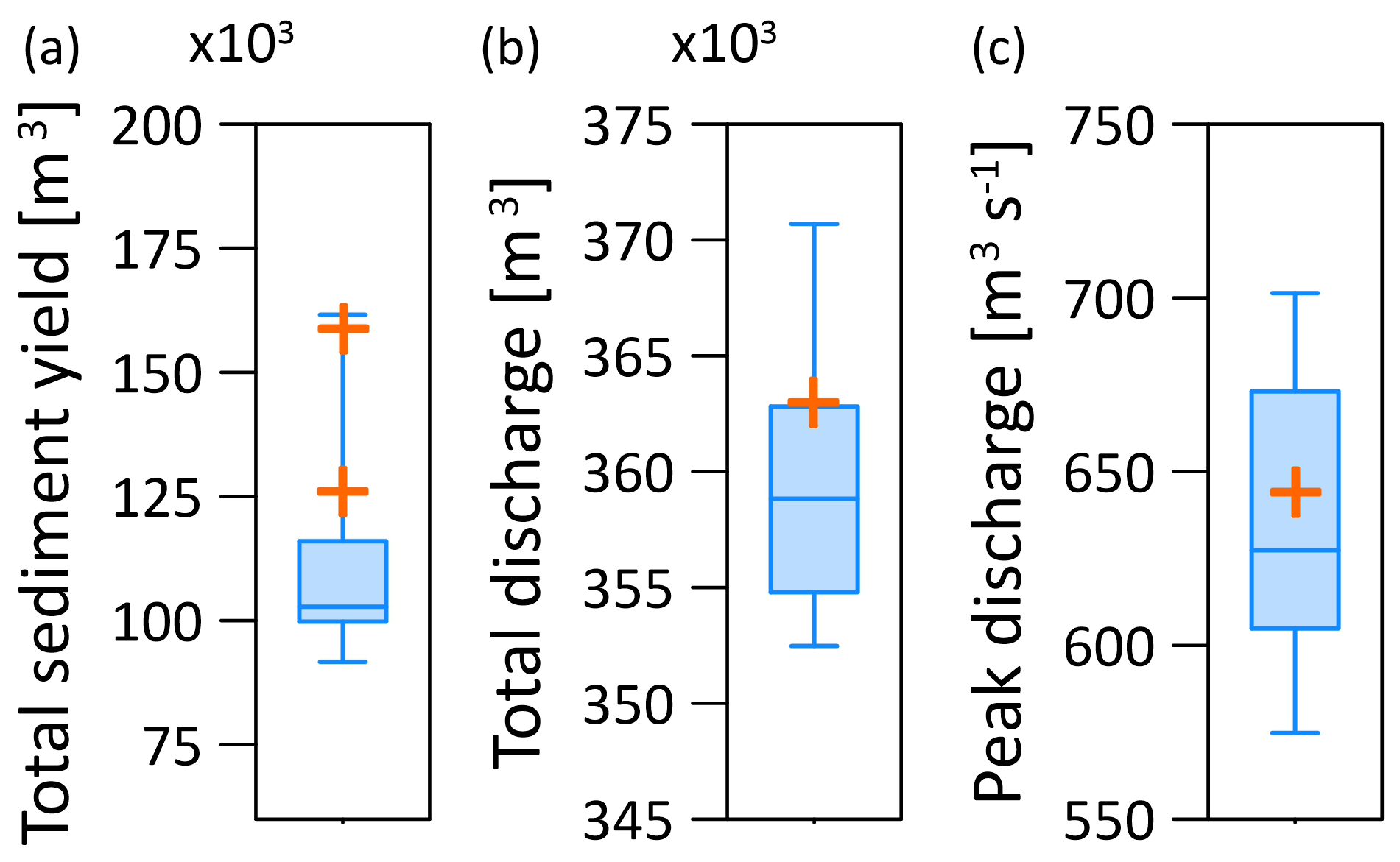
Figure 7Box plots showing the median (horizontal line), 25th–75th percentile range (shaded area), and maximum and minimum range (bounded with lines) of the total sediment yield (a), total streamflow volume (b), and peak streamflow (c) from the 10 downscaled spatial rainfall realizations for the heavy rainfall event of August 2005. The orange “+” symbols represent the observed data for the total and peak streamflow and the estimated range of the total sediment yield.

Download

The impacts of the changes in the spatial structure of heavy rainfall are expressed on bed load and suspended sediment load. For the August 2005 event, the volume of the sediment transport at the outlet of the catchment (minus the observed volume estimated for the lateral erosion that is not simulated by the model) was estimated between 125 000 m³ (Bezzola and Hegg, 2008) and 160 000 m³ (Rickenmann et al., 2016; Rickenmann and Koschni, 2010). Most simulated realizations underestimate the reported volumes (25th–75th percentile range, Fig. 7), yet two of the realizations do fall within this range (simulating 128 620 and 161 600 m³ of sediment yield).

Each individual simulation of the design storm experiment runs for an 8 d period. The first 4 d are used as a spin-up period to stabilize the streamflow at the outlet of the catchment for a baseflow of 10 m³ s⁻¹, which is similar to the observed value. Consequently, model output analysis and performance metrics for these simulations were computed after day 4.

4.1 Stratiform rainfall type

Peak streamflow and sediment yield – as expected – are predicted to enhance (reduce) with increasing (decreasing) rainfall amounts; however, the peaks were found to be mainly sensitive to the changes in the mean areal rainfall, since changing rainfall peak intensity only did not affect streamflow considerably. For example, examining the results for ΔT=4 ^∘C in Fig. 8, an increase of the mean areal rainfall by 7 % ^∘C⁻¹ resulted in an increase in peak streamflow by 62 %, an increase of the mean areal rainfall at a rate of 3 % ^∘C⁻¹ resulted in an increase in peak streamflow by 25 %, and a decrease in the mean areal rainfall at a rate of −3 % ^∘C⁻¹ resulted in a decrease in peak streamflow by −18 %. The peak sediment yield also showed higher sensitivity to changes in mean areal rainfall (Fig. 8, changes to the symbol sizes). For example, for ΔT=4 ^∘C, an increase of the mean areal rainfall by 7 % ^∘C⁻¹ and 3 % ^∘C⁻¹ resulted in an increase of 210 % and 84 %, respectively, in the peak sediment yield, and a decrease in the mean areal rainfall at a rate of −3 % ^∘C⁻¹ resulted in a decrease in sediment yield peak by −31 %, underlining how non-linearities in sediment transport are much stronger than for discharge.

Focusing on the results where the peak rainfall intensity at the grid scale is intensifying by 7 % ^∘C⁻¹ but the mean areal rainfall remains unchanged (Fig. 8, orange symbols) reveals different sensitivities for the peak streamflow and peak sediment yield. Although the peak rainfall at the grid scale intensified, peak streamflow is hardly affected; the maximum enhancement is 2 % for the ΔT=4 ^∘C scenario, which is almost negligible. However, the intensification of the peak rainfall at the grid scale resulted in a considerable enhancement of the peak sediment yield of 4 % for ΔT=1 ^∘C, 8 % for ΔT=2 ^∘C, 11.8 % for ΔT=3 ^∘C, and 16.4 % for ΔT=4 ^∘C (Fig. 8).

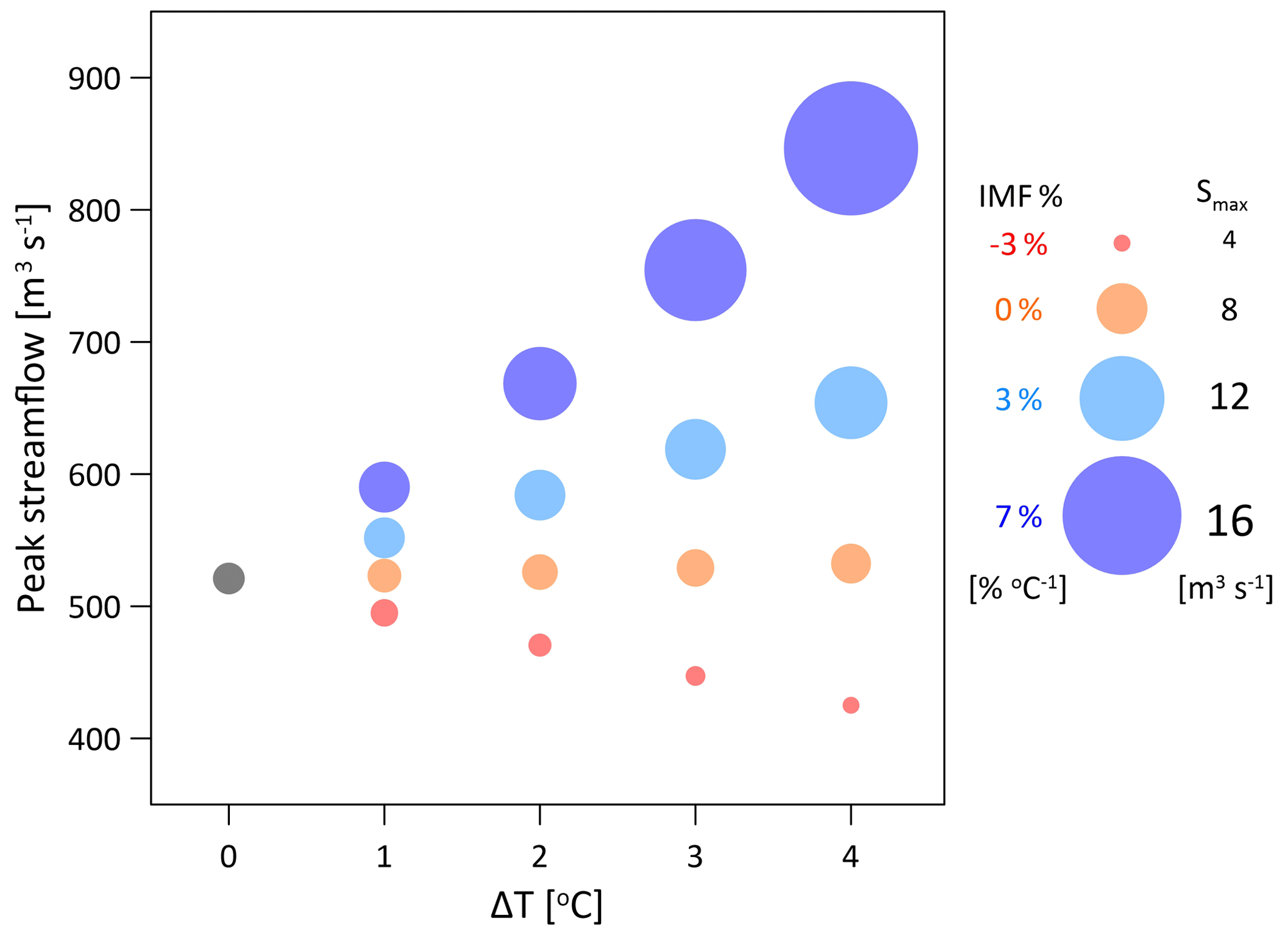
Figure 8Response of the peak streamflow (y axis) and peak sediment yield (symbol size, S_max) at the outlet of the catchment to changes in the rainfall spatial structure with temperature for stratiform rainfall type. Peak rainfall intensity increases by 7 % ^∘C⁻¹ for all points. Different colours represent a mean areal rainfall intensity change: decrease of −3 % ^∘C⁻¹ (red), not changing (orange), increase of 3 % ^∘C⁻¹ (blue), and increase of 7 % ^∘C⁻¹ (dark blue). Reference (base scenario) for the sensitivity is the single point at ΔT=0 (grey).

Download

Similar sensitivities were found when examining the effects of the intensification of the peak rainfall intensity at the grid scale on total streamflow and sediment yield, assuming no changes to the mean areal rainfall (case 2). While total streamflow changed by less than 1 % for the different temperature scenarios, total sediment yields increased by 2 %, 4 %, 7 %, and 9 % for the ΔT=1 to 4 ^∘C scenarios, respectively. However, modifying the mean areal rainfall, even by simply applying ±3 % ^∘C⁻¹, resulted in a change to the total sediment yields higher than 10 % (Fig. 9).

The geomorphic multiplier implies a non-linear relation between total streamflow and total sediment yield (Coulthard et al., 2012b). Plotting these two quantities against each other (Fig. 9), using information from all the scenarios, the sensitivity of the geomorphic multiplier to changes in the rainfall spatial structure can be shown. The relation between the simulated total sediment yield and total streamflow were found to follow a power law once fitted to the actual simulated values of the total streamflow and sediment yield (R²=0.99, not shown), which is closely correlated to the changes in total rainfall amounts (ΔP, symbol size). Most points fall directly along the fitted line – which implies that the total streamflow and total sediment yield are mainly sensitive to changes in the total rainfall volume. Points that deviate from the fitted line, e.g. the scatter of dots along the y axis close to the 0 % change in total streamflow, have different spatial structures of rainfall. The sensitivity of the total sediment yield to changes in the rainfall spatial structure, due to the intensification of peak rainfall intensity or due to different rainfall spatial correlation structures is estimated to be of the order of ±10 % (of the reference total sediment yield).

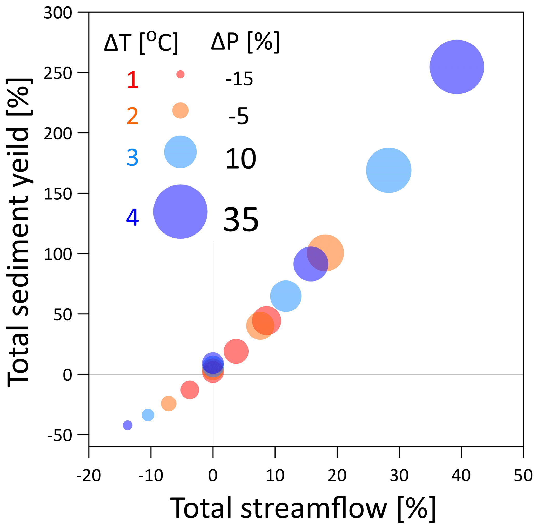
Figure 9Changes in the total sediment yield (y axis) as a function of the changes in total streamflow (x axis) in relation to the changes in total rainfall amounts (symbol size, ΔP for stratiform rainfall type). The relevant temperature scenario (ΔT) is expressed by the colour of the symbols (1 ^∘C – red, 2 ^∘C – orange, 3 ^∘C – blue, and 4 ^∘C – dark blue). The reference to compute the changes is the total streamflow and sediment transport of the base scenario (at ΔT=0).

Download

The spatial sensitivity of the hydro-morphological response was lastly examined by means of two spatial indices: (i) the maximum inundated area for each realization, defined as the total area with water levels higher than 1 cm, which represents the area of overland flow on hillslopes and flow in channels and (ii) the total area of erosion or deposition (active area from hereafter), defined by comparing the elevation map at the end of the realization to the pre-storm elevation map and summing the grid cells where net erosion or deposition occurred (i.e. grid cells with elevation difference greater than 1 cm; see example in Fig. S3). Both the maximum inundated area and active area were found to react to the changes in mean areal rainfall intensity. An increase in areal rainfall amounts and in the area of heavy rainfall resulted in an increase in both the maximum inundated and active areas (IMF % =3 % and 7%, Fig. 10), while a decrease in areal rainfall amounts and in the area of heavy rainfall resulted in a decrease in both (IMF % $=-\mathrm{3}$ %, Fig. 10). The maximum inundated area and active area has a different sensitivity to the intensification of peak rainfall intensity for the case when the mean areal rainfall remain unchanged (case 2, IMF % =0 %). In this case the maximum inundated area was found to slightly decrease from 54.5 km² for ΔT=0 ^∘C to 54.3 km² for ΔT=4 ^∘C (Fig. 10a) – practically remaining unchanged (less than 1 % change), while the active area was found to increase from 67.6 km² for ΔT=0 ^∘C to 71 km² (+5 %) for ΔT=4 ^∘C (Fig. 10b).

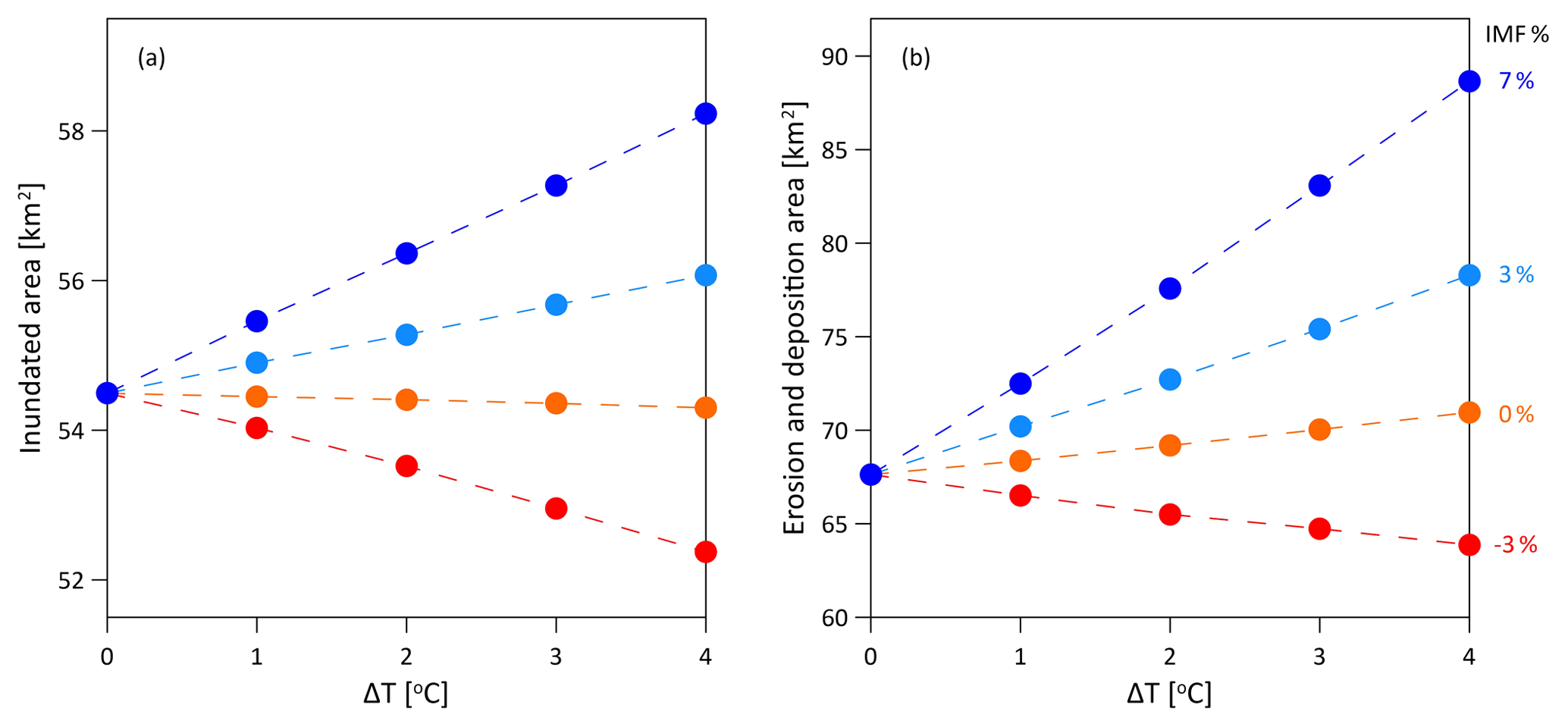
Figure 10The sensitivity of the maximum inundated area (a) and the active erosion plus deposition area (b) to changes in the rainfall spatial structure with temperature for stratiform rainfall type. Peak rainfall intensity increases by 7 % ^∘C⁻¹ for all points. Different colours represent mean areal rainfall intensity decrease of −3 % ^∘C⁻¹ (red), not changing (orange), increases of 3 % ^∘C⁻¹ (blue), and increases of 7 % ^∘C⁻¹ (dark blue). Reference (base scenario) for the sensitivity is the point at ΔT=0.

Download

4.2 Convective rainfall type

The hydro-morphological response driven by convective rainfall was compared to the response obtained with the stratiform rainfall experiment. Similar trends for the hydro-morphological response were found for the two rainfall types; however, magnitudes were different for some of the examined components. Differences in the hydro-morphological response for the ΔT=2 ^∘C scenario between the two rainfall types were compared for cases 1 to 3 (Table 4). The hydro-morphological response for the scenario in which both the peak rainfall intensity and mean areal rainfall are intensifying (case 3) is similar for the two rainfall types (Table 4). For the case where the peak rainfall intensified while the mean areal rainfall intensity weakened (case 1), a more pronounced decrease (between the two rainfall types) in the peak streamflow, total sediment yield, and in the active area were found for the simulations with the stratiform rainfall type (Table 4). On the other hand, the decrease in the maximum inundated area and total streamflow were larger, and the response of the peak sediment yield had a different sign for the convective rainfall type (Table 4).

Table 4The hydro-morphological response produced by stratiform and convective rainfall types for the ΔT=2 ^∘C scenario in comparison to the reference scenario (ΔT=0 ^∘C).

Download Print Version | Download XLSX

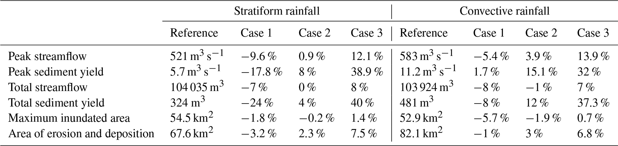
Differences in the hydro-morphological response were also found for case 2 (no change in areal rainfall, Table 4). While for the stratiform rainfall the peak streamflow remains unchanged and a small increase in the peak sediment yield was reported, for the convective rainfall both peaks considerably increased. The streamflow volume remains unchanged for both rainfall types, while the enhancement of the total sediment yield was found to be more pronounced for the convective rainfall type. As for the stratiform rainfall, the streamflow volume and total sediment yield simulated with the convective rainfall are related by a power law relation ($S=\mathrm{8.1}\times {\mathrm{10}}^{-\mathrm{17}}{Q}^{\mathrm{3.7}}$ and $S=\mathrm{6.5}\times {\mathrm{10}}^{-\mathrm{13}}{Q}^{\mathrm{3}}$ for stratiform and convective rainfalls, respectively, where S is total sediment yield and Q is total discharge, R²=0.99 for both cases). The difference in the exponential relations between the two rainfall types implies that the geomorphic multiplier, besides being dependent on the catchment characteristics and sediment supply, depends to a certain extent on rainfall structure as well.

4.3 Summary of the CC experiment

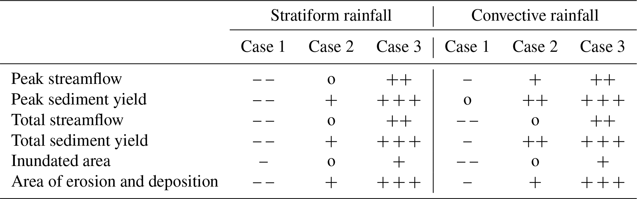
A qualitative summary of the sensitivity of the hydro-morphologic response to the two rainfall types is presented in Table 5.

The response of the hydrological component ranges from no response (stratiform rainfall) to low positive response (convective rainfall) for the case where intensification of the peak rainfall intensity at the grid scale is the only change considered (case 2), with a low (stratiform) to medium (convective) positive response for the geomorphological components. The response is markedly positive for an increase in the mean areal rainfall (case 3) for both rainfall types, with a medium enhancement of streamflow volume and peaks and high enhancement of sediment peak and total yield. The response for a decrease in the mean areal rainfall (case 1) is toward a decrease of the analysed variables, but differences can be observed for the two rainfall types. For stratiform rainfall, both the hydrological and geomorphological variables showed a medium negative response, while for the convective rainfall a medium negative response was detected for the hydrological variables but a milder negative response was found for the geomorphological ones. Results demonstrated that the hydro-morphological response is sensitive to the rainfall spatial structure as conditioned on the rainfall type, even though rainfall volume remains the most important factor.

Table 5A qualitative summary of the hydro-morphological response to the three main studied cases (Fig. 1) for the rainfall spatial structure corresponding to stratiform and convective types. For all three cases, the peak rainfall intensity at the grid scale intensifies. Case (1) total rainfall amount decreases, area of heavy rainfall decreases; case (2) total rainfall amount remains unchanged and area of heavy rainfall slightly decreases; case (3) total rainfall amount increases and area of heavy rainfall increases. The response varies between a strong negative response (– – –), no change (o), and a strong positive response ($+++$).

Download Print Version | Download XLSX

4.4 2CC experiment

Enhancements in the peak streamflow and peak sediment yield were found when increasing the peak rainfall intensity with temperature using a 2CC scaling in the convective storm experiment while preserving the mean areal rainfall. For example, for ΔT=1 ^∘C, the peak streamflow moderately increased from 583 m³ s⁻¹ (reference) to 593 m³ s⁻¹ (CC) and 604 m³ s⁻¹ (2CC), while the peak sediment yield increased from 11.2 m³ s⁻¹ (reference) to 12 m³ s⁻¹ (CC) and 12.8 m³ s⁻¹ (2CC). In addition, a subtle decrease in the streamflow volume and a considerable increase in the total sediment yield were observed, respectively reducing from 103 924 m³ (reference) to 103 326 m³ (2CC) and increasing from 481 m³ (reference) to 535 m³ (2CC). A decrease was found for the maximum inundated area, from 52.9 km² (reference) to 51.9 km² (2CC), while an increase was observed for the active area, from 82.1 km² (reference) to 84.5 km² (2CC).

5.1 Physical interpretation of the hydro-morphological responses

As expected, intensification of the peak and mean areal rainfall lead to a higher streamflow peak because the total amount of rainfall considerably increases (Table 4, case 3). However, localized intensifications of the peak rainfall alone, without changes to the total rainfall amounts (case 2), do not necessarily enhance the peak streamflow as the intensification of the peak rainfall is associated with a decrease in the area of the heavy rainfall over the entire rainfall field to preserve the rainfall volume. Stratiform rainfall fields are characterized by relatively high spatial correlation in space that is not changing dramatically between the reference and design scenarios (e.g. Fig. 4). That means that the local intensification of heavy rainfall and decrease of the area of heavy rainfall over the rainfall fields results in minor changes to the volume of rainfall that is reaching the catchment at a given time, thus the peak streamflow remains largely unchanged (e.g. Bell and Moore, 2000; Gupta et al., 1996; Kalinga and Gan, 2006). However, for convective rainfall, the change in rainfall spatial structure is expressed by generating high-intensity convective features (Haerter, 2019; Haerter et al., 2017) that are contributing higher volumes of rainfall to specific parts of the catchment in shorter durations, resulting in an enhancement of runoff and peak streamflow (e.g. Morin et al., 2006; Peleg et al., 2015; Yakir and Morin, 2011). When the mean areal rainfall is decreasing but the peak rainfall is intensifying (Table 4, case 1), for both stratiform and convective rainfall we observed a decrease in the peak streamflow due to the lower rainfall volumes but such a decrease is much less pronounced for convective rainfall.

Unsurprisingly, the changes in streamflow volume are following the changes in the total rainfall volume, which are expressed by changes in mean areal rainfall (Table 4, cases 1 and 3). However, the streamflow volume is not sensitive to the intensification of the peak rainfall by itself (case 2), as negligible (less than 1 %) changes in streamflow volume were produced. Similarly, the maximum inundated area was found to be sensitive mainly to the changes in the mean areal rainfall and therefore rainfall volume. A larger decrease in the inundated area is observed for the convective rainfall in comparison to the stratiform rainfall (Table 4, case 1). This is related to the fact that intense convective rainfall features vary significantly in space and sometimes are not covering the entire catchment, in such a case not all tributaries are affected by the heavy rainfall (Goodrich et al., 1995; Lopes, 1996), and the total inundated area tends to decrease.

The geomorphological variables, peak and total sediment yield, and area of erosion or deposition were found to be more sensitive to changes in rainfall structure itself in comparison to the hydrological variables (Table 4). This is related to the geomorphic multiplier, i.e. the capacity of sediment transport to respond disproportionally to a change in the hydrological regime, and it is the outcome of processes, which are triggered only when certain thresholds are exceeded. The intensification of the peak rainfall intensity at the grid scale alone (case 2) explains part of the response, as higher rainfall rates are expected to enhance soil erosion (Nearing et al., 2004, 2005; Shen et al., 2016) and trigger more landslides and debris flows (Guzzetti et al., 2008; Iverson, 2000; Leonarduzzi et al., 2017). Although not explicitly exploring the geomorphological response at the storm scale, Coulthard et al. (2012b), Coulthard and Skinner (2016), and Deal et al. (2017) discussed already the role of local extreme rainfall intensity in enhancing erosion and accelerating landscape evolution. Adding to their conclusions, it is clear that the geomorphological response is sensitive to the rainfall type as intense convective rainfall features enhance the geomorphological response (Table 4, case 2).

5.2 Implications for climate change impact studies

Results imply that the hydro-morphological response of medium-sized catchments is influenced by changes in the rainfall spatial structure at small scale, and, due to above-mentioned threshold effects, the geomorphological variables are more sensitive to changes in rainfall structure than the hydrological variables. Various representative cases of changes in rainfall spatial structure with increasing temperature were explored in order to study the sensitivity of the fluvial system to these changes. We note that the changes in rainfall structure can be more complex than schematized in this work. For example, Wasko et al. (2016) showed that the intensification of the peak rainfall is associated with a reduction in the area of the storm and with an intensification of the mean areal rainfall but at a lower rate than the intensification in the rainfall peak. Additionally, the relations between the rainfall spatial structure and temperatures were observed so far only in a few locations worldwide (Lochbihler et al., 2017; Peleg et al., 2018b; Wasko et al., 2016), and they remain unknown for most locations.

Representing spatial rainfall structures requires high-resolution simulations. In hydrology, using gridded rainfall data for climate change impact studies is becoming common practice. In recent years, there has been an increase in the availability of distributed hydrological models (Fatichi et al., 2016; Paniconi and Putti, 2015), and they have been used in the context of climate impacts (e.g. Dams et al., 2015; Fatichi et al., 2015; Perra et al., 2018). However, this is much less the case for geomorphological impacts (e.g. Francipane et al., 2015; Pandey et al., 2016; Ramsankaran et al., 2013; Zi et al., 2016), where the added value of using high-resolution gridded rainfall data for climate change impact studies is still not widely explored (Li and Fang, 2016) and most LEMs do not receive distributed rainfall as input (Coulthard and Skinner, 2016; Tucker and Hancock, 2010). The risk of over-predicting the geomorphological response is significantly increased when using uniform rainfall instead of distributed rainfall. This was discussed by Coulthard and Skinner (2016) and here we demonstrate plausible consequences of global warming on the spatial rainfall structure and its potential impacts. Specifically, case 4 represents the situation where both peak rainfall intensity and mean areal intensity are assumed to intensify at the same rate, meaning that the rainfall amounts are increasing while the rainfall spatial structure remains largely unchanged. In the context of a climate change study, using case 4 would be equivalent to using the observed rainfall and increasing the rainfall amounts evenly over the catchment in response to climate change. The peaks of streamflow and sediment yield (Fig. 8), streamflow volume and total sediment yield (Fig. 9), and inundated area and active area (Fig. 10) – all these quantities – will be over-predicted for such a case in comparison to other scenarios, where the areal and peak rainfall intensities, and thus the rainfall spatial structure, are changing at different rates. This also emphasizes the importance of using either high-resolution CPMs to simulate changes in the rainfall for the future climate or appropriate downscaling of the rainfall simulations from climate models. If downscaling is based on simple relationships between rainfall and temperature that are measured at the point scale (i.e. using ground stations), results must be analysed with care, as often these relationships are extrapolated to a much larger (catchment) scale (Dahm et al., 2019; Fadhel et al., 2018; Lenderink and Attema, 2015). A viable alternative is presented here. It is represented by space-time rainfall generators, which allow for downscaling of the rainfall to the required space-time resolution while maintaining realistic spatial characteristics of rainfall fields based on current observations at a point and weather radar scales and factors of change derived from climate models (e.g. Peleg et al., 2019).

5.3 Generalization and limitations of the numerical experiment

The presented study offers a quantification of the effects of different spatial structures of rainfall using 10 stochastic realizations and their effects on key hydro-morphological variables, but it also refers to a single design storm, a single catchment, and only one LEM. The design storm represents a realistic storm in terms of rainfall amount, but it is simplified in terms of the temporal evolution, which can affect the fluvial response (Istanbulluoglu and Bras, 2006; Tucker and Bras, 2000). Furthermore, the storm is advected with a fixed velocity and direction, and the rainfall is assumed to cover the entire catchment – assumptions that can affect the hydrograph peak, volume, and timing (Morin et al., 2006; Singh, 1997; Yakir and Morin, 2011). The LEM was used with a simplified setup that does not include vegetation–erosion interactions and lateral erosion; concurrently, the hydrological module is not representing all of the hydrological processes, such as changes in soil saturation and infiltration capacity, which can be important for precise estimation of the hydro-morphological response (Coulthard et al., 2013; Paschalis et al., 2014; Tucker and Hancock, 2010). The TOPMODEL formulation of runoff production, controlled exclusively by the saturated area that is proportional to the rainfall volume, scales the streamflow volume almost linearly with the rainfall volume. Alternative representations of runoff production that are more realistic may provide a more pronounced non-linear response of the hydrology of the catchment and therefore emphasize the role of rainfall spatial variability. However, the LEM validation proved that the model simulates streamflow and sediment yield satisfactorily for the examined 15 d period, which generates confidence in the overall predictions.

Even though we use a single catchment, the Kleine Emme catchment can be considered representative of an average Alpine catchment in terms of elevation, land use, and stream morphology, and the sensitivities of the hydro-morphological response to different spatial representations of heavy rainfall found in this study are likely indicative of the behaviour of other medium-sized mountainous catchments. Extrapolations for other climatic regions, rainfall regimes, and catchments with a different topography and geomorphology are instead highly speculative.

In this study, we considered sediment yield at the outlet of the catchment and the total area of erosion and deposition within the catchment as a representative function of the geomorphic change to rainfall structure. Internal geomorphological changes (see Skinner et al., 2018) can be explored and can be the subject of future work.

Finally, while we studied the small-scale spatial structure of rainfall, additional research is needed in order to understand the sensitivity of the catchment to the rainfall temporal structure at fine scale and its relative importance when compared to spatial structure in shaping the landscape over long (millennial) periods.