the Creative Commons Attribution 4.0 License.
the Creative Commons Attribution 4.0 License.
 | 26 May 2020
Short communication: Landlab v2.0: a software package for Earth surface dynamics
Katherine R. Barnhart
Eric W. H. Hutton
Gregory E. Tucker
Nicole M. Gasparini
Erkan Istanbulluoglu
Daniel E. J. Hobley
Nathan J. Lyons
Margaux Mouchene
Sai Siddhartha Nudurupati
Jordan M. Adams
Christina Bandaragoda
Numerical simulation of the form and characteristics of Earth's surface provides insight into its evolution. Landlab is an open-source Python package that contains modularized elements of numerical models for Earth's surface, thus reducing time required for researchers to create new or reimplement existing models. Landlab contains a gridding engine which represents the model domain as a dual graph of structured quadrilaterals (e.g., raster) or irregular Voronoi polygon–Delaunay triangle mesh (e.g., regular hexagons, radially symmetric meshes, and fully irregular meshes). Landlab also contains components – modular implementations of single physical processes – and a suite of utilities that support numerical methods, input/output, and visualization. This contribution describes package development since version 1.0 and backward-compatibility-breaking changes that necessitate the new major release, version 2.0. Substantial changes include refactoring the grid, improving the component standard interface, dropping Python 2 support, and creating 31 new components – for a total of 58 components in the Landlab package. We describe reasons why many changes were made in order to provide insight for designers of future packages. We conclude by discussing lessons about the dynamics of scientific software development gained from the experience of using, developing, maintaining, and teaching with Landlab.
- Article
(3121 KB) - Full-text XML
- BibTeX
- EndNote


Landlab is a Python package to support the creation of numerical models in Earth surface dynamics. Numerical models support researchers to simulate past, present, and future dynamics of a system. This enables conceptual model validation, testing of alternative hypotheses, and prediction under uncertainty. Numerical modeling is especially important for Earth surface dynamics because of the timescale mismatch between human observation and system evolution. Landlab is an open-source Python-language package that provides the common elements of infrastructure needed to support the creation of new models. These include a model domain representation (the model grid), physical process components, and utilities that support use and extension of the package. Landlab's modular design lowers the barriers of entry to computational research, reduces researcher time, and supports publication of reproducible scientific research products (e.g., Bandaragoda et al., 2019). Development and maintenance of Landlab follows modern software development standards such as version control, integrated testing and documentation, continuous integration, and multiplatform binary distribution (e.g., Adorf et al., 2019; Hwang et al., 2017; Mandli et al., 2016; Poisot, 2015; Taschuk and Wilson, 2017; Wilson et al., 2014). Our open-source development and use of semantic versioning (SemVer 2.0.0, https://semver.org, last access: 12 May 2020) provides a necessary but not sufficient tool for reproducible research in Earth surface dynamics (e.g., Chen et al., 2018).
Landlab was designed as a key element in the Community Surface Dynamics Modeling System (CSDMS) suite of tools (Peckham et al., 2013). Initial development of Landlab began in 2012 and culminated in a version 1.0 release (referred to as v1.0) described by Hobley et al. (2017). Figure 1 provides examples of the breadth of modeling efforts implemented with Landlab.
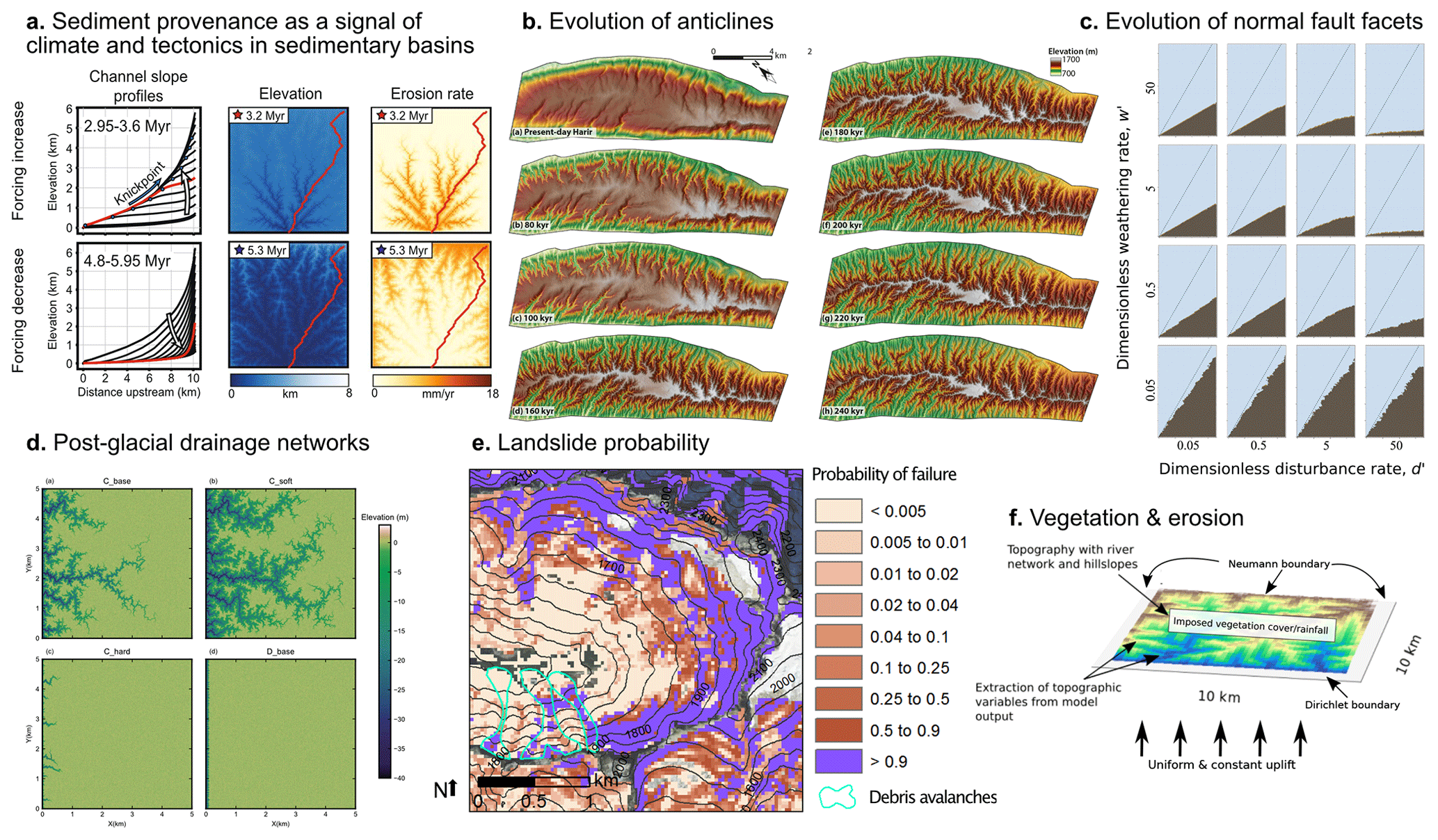
Figure 1Examples of modeling applications implemented with Landlab span a wide range of timescales and topics. A recent selection of examples intended to highlight diversity of applications includes the following examples: (a) sediment provenance studies (Sharman et al., 2019, reproduction modified from their Fig. 2), (b) landscape evolution of anticlines (Zebari et al., 2019, reproduction of their Fig. 8), (c) cellular automaton simulation of normal fault facets (Tucker et al., 2020, reproduction of their Fig. 9), (d) the evolution of post-glacial drainage networks (Lai and Anders, 2018, reproduction of their Fig. 4), (e) estimates of landslide probability (Strauch et al., 2018, reproduction modified from their Fig. 9), (f) and coevolution of vegetation and erosion (Schmid et al., 2018, reproduction of their Fig. 3). All subpanels except (d) covered by CC BY license. Permission to reproduce (d) was obtained through Copyright Clearance Center RightsLink.
Subsequent to the release of v1.0, the core development team and many community members have contributed additional features and bug fixes to the software. Based on experience using and developing with Landlab, the development team identified changes to Landlab that were not backwards compatible, indicating a major release was necessary to convey to Landlab users to expect substantial changes. This motivated the creation of Landlab v2.0, the focus of this contribution. A new major version was needed to support (a) backward-compatibility-breaking changes associated with refactoring core data structures and (b) removal of support below Python version 3.
The scope of this contribution is to review the core concepts that underpin Landlab's design (Sect. 3), describe the changes and new features added since v1.0 (Sect. 4), discuss citation of software (Sect. 5), and document lessons we have learned about community software development from developing and maintaining Landlab (Sect. 6). Before concluding we provide recommendations for those interested in being involved with Landlab (Sect. 7). We note that while much of the contribution discusses general issues of scientific software development, Sect. 4 is inherently specific to Landlab and describes technical details of changes between v1.0 and v2.0. For a comprehensive description of the design and theory behind Landlab v1.0 the reader is referred to Hobley et al. (2017). Additionally, we will not present detailed description of the use of the software, discuss numerical methods, or review the literature that supports each process implemented in Landlab. In general, methods and supporting literature can be found in key publications introducing each component (see Sect. 5), and guidance on software usage can be found on the Landlab website.
The design of the Landlab package, its development practices, and the changes made in v2.0 are best understood in light of the three audiences who interact with the package. Unlike software that is developed by dedicated software engineers who may not use the software themselves, Landlab developers also use the software for their research and teaching. Thus, the first audience is user-developers, people who extend, modify, or otherwise contribute to the source code in order to accomplish their goals. Notably, most Landlab user-developers have little to no background in software engineering. The second audience is users: people who use Landlab to write their own programs but do not modify or contribute to Landlab's source code. Among this group, it is natural for some to transition to becoming user-developers, who contribute new components or utilities to the main Landlab code base. The final audience is teachers–students, people who use Landlab in an instructional classroom setting as part of a course.
In creating the source code, writing the documentation, determining the development practices, and maintaining the package, the needs, abilities, and time constraints of all three audiences must be balanced. This is particularly important for packages like Landlab with a small active developer community (n<20) and a research-scale user community (e.g., tens to hundreds of researchers and perhaps a few thousand students over the lifetime of the software, rather than millions of users). Our approach is to adopt many of the key design principles underlying modern academic software design best practice (e.g., Wilson et al., 2017; Turing Way Community et al., 2019). These include an extensive automatic test suite, integrated documentation, version control, continuous integration, lint checking, and releasing binary packages for users. These design choices were made to ensure that Landlab is sustainable into the future to support the user–developer–learner communities (see Hobley et al., 2017). Community contributors play an important role in developing community open-source software. Two of their most important roles are improving and refining documentation when it is unclear and identifying software bugs. Because Landlab currently has a relatively small user base with limited experience contributing to documentation, it takes longer (months to years) for documentation to be refined by users compared to software with more users (days to months). The relatively long “refinement residence time” means that a commitment to high-quality tests is critically important (see Sect. 6.1).
A core design principle behind the Landlab package is modularity. Separating the elements of a numerical model into reusable parts decreases the human time associated with creating a new model or extending a current one. The design of Landlab is discussed extensively in Hobley et al. (2017). Here we briefly summarize the key points to provide context to the changes and new features that are discussed further in Sect. 4.
The modular design of Landlab comprises the following categories of software infrastructure:
-
Model grids: data structures implemented as Python classes that represent the computational domain, connectivity between parts of the domain, and provide a centralized location to store state variables.
-
Utilities: functions that provide solutions to common problems (e.g., numerical functions for gradients, mapping, and flux divergence; basic plotting; watershed delineation; and file input/output).
-
Components: representation of core surface processes (e.g., stream power, flow accumulation, and precipitation) as a Python class with a common interface.
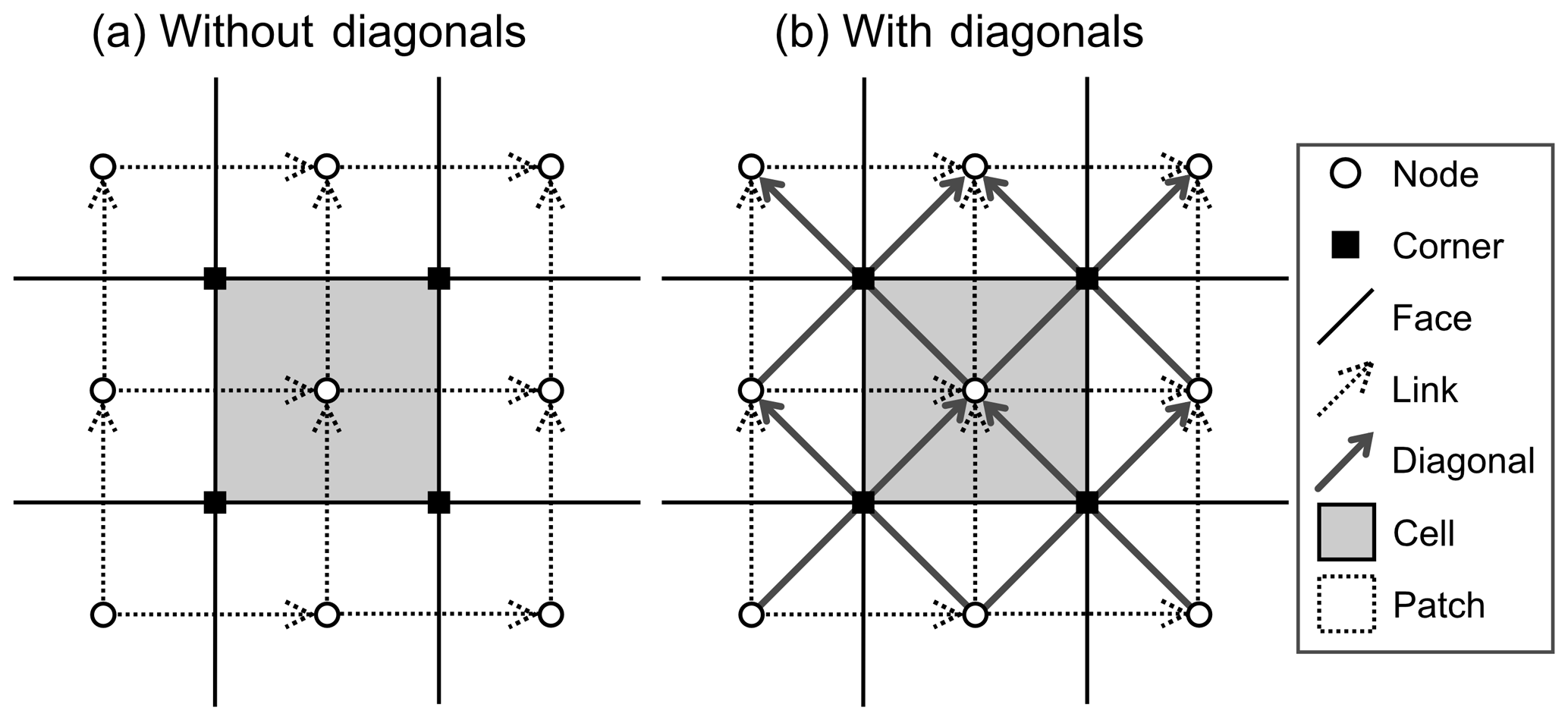
The grid represents a 2-D domain as a dual graph. Each graph in the dual graph is a set of points, connected by lines, and outlining polygons. The two graphs are offset from one another such that the points of one graph are located inside of the polygons of the other graph. Each graph is a planar graph, meaning that the lines connecting points do not cross. In Landlab, we refer to the first graph as composed of nodes connected by links which outline patches. Corners are located inside patches and are connected by faces, which outline cells. With this framework, data identified at a given point in space have both a connectivity to other points defined by its lines and a uniquely associated spatial area and set of bounding edges drawn the from enclosing polygon in the other graph (Fig. 2).
There are four aspects of the grid that are worth highlighting. First is that the Landlab model grids provide information about the connectivity and adjacency of all grid elements (nodes, links, patches, corners, faces, and cells). Second, the model grids use a consistent framework for the numbering of grid elements and identifying a direction for each link and face (note that this is a topologic direction based on the orientation of the link in x–y space, not a flow direction). This permits consistent application of numerical methods based on grid element ID that may be transferred to grids of different shapes and sizes.
Third, Landlab supports regular and irregular model grids through the same interface. The Landlab model grid library includes data structures for networks, regular rasters, general irregular meshes (Voronoi cells with Delaunay triangulated nodes), regular hexagons, and radially symmetric irregular meshes. Landlab v2.0 assumes all links and faces are straight. The model grids were designed to accommodate extension to more exotic 2-D geometries.
Finally, the model grid may be used to store data fields at any grid element. Fields represent state variables and are useful when multiple components use or modify the state variables. When a field is stored on the grid, Landlab enforces characteristics such as the number of elements and provides the ability to use adjacency information associated with the grid.
The Landlab model grids keep track of boundary conditions using arrays of integers with flags indicating characteristics such as fixed-value, fixed-gradient, or closed to flux (grid.status_at_X where X is the name of the grid element). Note that we will use preformatted style text to indicate Landlab syntax. Thus far, most applications with Landlab use nodes and links as the primary grid elements. Thus, sets of standard boundary condition flags are presently only implemented for these two types of grid elements.
Utilities fall into two subcategories: general numerical utilities and application-focused utilities. In the first category are general functions to calculate quantities such as gradients or flux divergence and map values from one grid element to another. Development has created numerical utilities focused on finite-difference/volume numerical solutions to differential equations and cellular automaton applications. The focus on finite-difference and finite-volume utilities, however, reflects the interests of developers rather than the potential characteristics of the package. In the second category are application-focused utilities. These utilities are typically developed for use in a particular component but have grown to have broader use within the package. For example the watershed utility submodule was developed to support the SpeciesEvolver but provides the broadly applicable ability to label watersheds.
Components are Python objects with a standard interface that implement a single Earth surface process, set of equations, or analysis compatible with the component interface (e.g., calculation of drainage density). All components require a Landlab model grid to instantiate and have a built-in function that advances the component forward in time or updates it based on the current values stored as fields. Components can be coupled by accessing and modifying the same fields stored on the model grid elements.
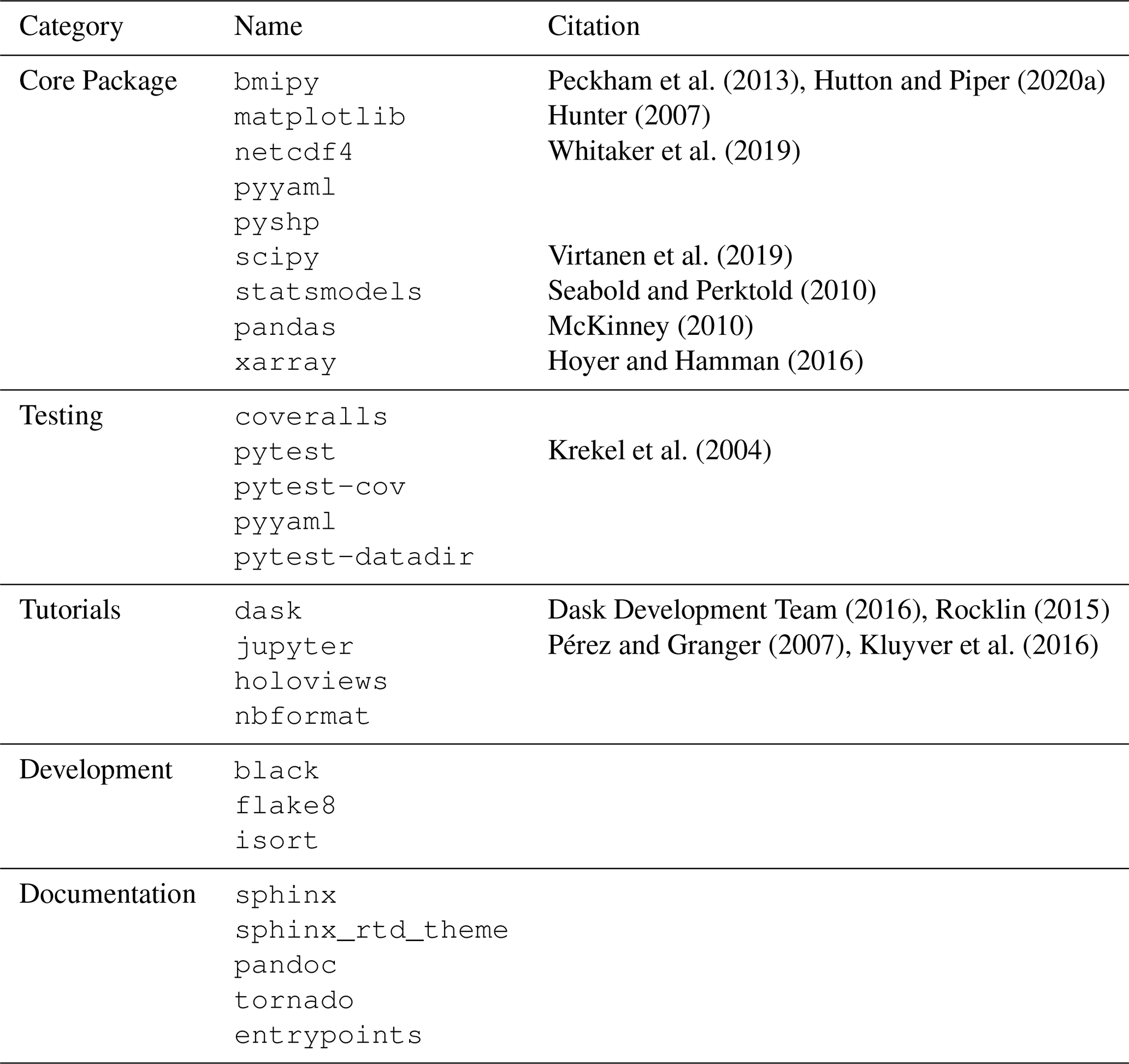
Landlab v2.0 contains many changes to the core source code that add new features. We have compiled tables describing the pre-existing, refactored, and new core capabilities of the Landlab package. These include data structures (Table 1), utilities (Table 2), new components (Table 3), and pre-existing or refactored components (Table 4). We list core package, development environment, testing, tutorial, and documentation dependencies in Table 5.
Barnhart et al. (2019b)Johnstone and Hilley (2015)Barnhart et al. (2019b)Johnstone and Hilley (2015)Ganti et al. (2012)Barnhart et al. (2019b)Davy and Lague (2009)Barnhart et al. (2019b)Ahnert (1976)Armstrong (1976)Braun and Willett (2013)O'Callaghan and Mark (1984)Tarboton (1997)Quinn et al. (1991)Freeman (1991)Litwin et al. (2020)Childs (1971)Marçais et al. (2017)Barnes et al. (2014)Strauch et al. (2018)Langston and Tucker (2018)Barnhart et al. (2018)Barnhart et al. (2018)Braun and Willett (2013)Barnes et al. (2014)Shobe et al. (2017)Singer et al. (2018)Lyons et al. (2020)Albert et al. (2016)Lyons et al. (2019)Barnhart et al. (2019b)Braun and Willett (2013)Barnhart et al. (2019b)Ganti et al. (2012)Davy and Lague (2009)Carretier et al. (2016)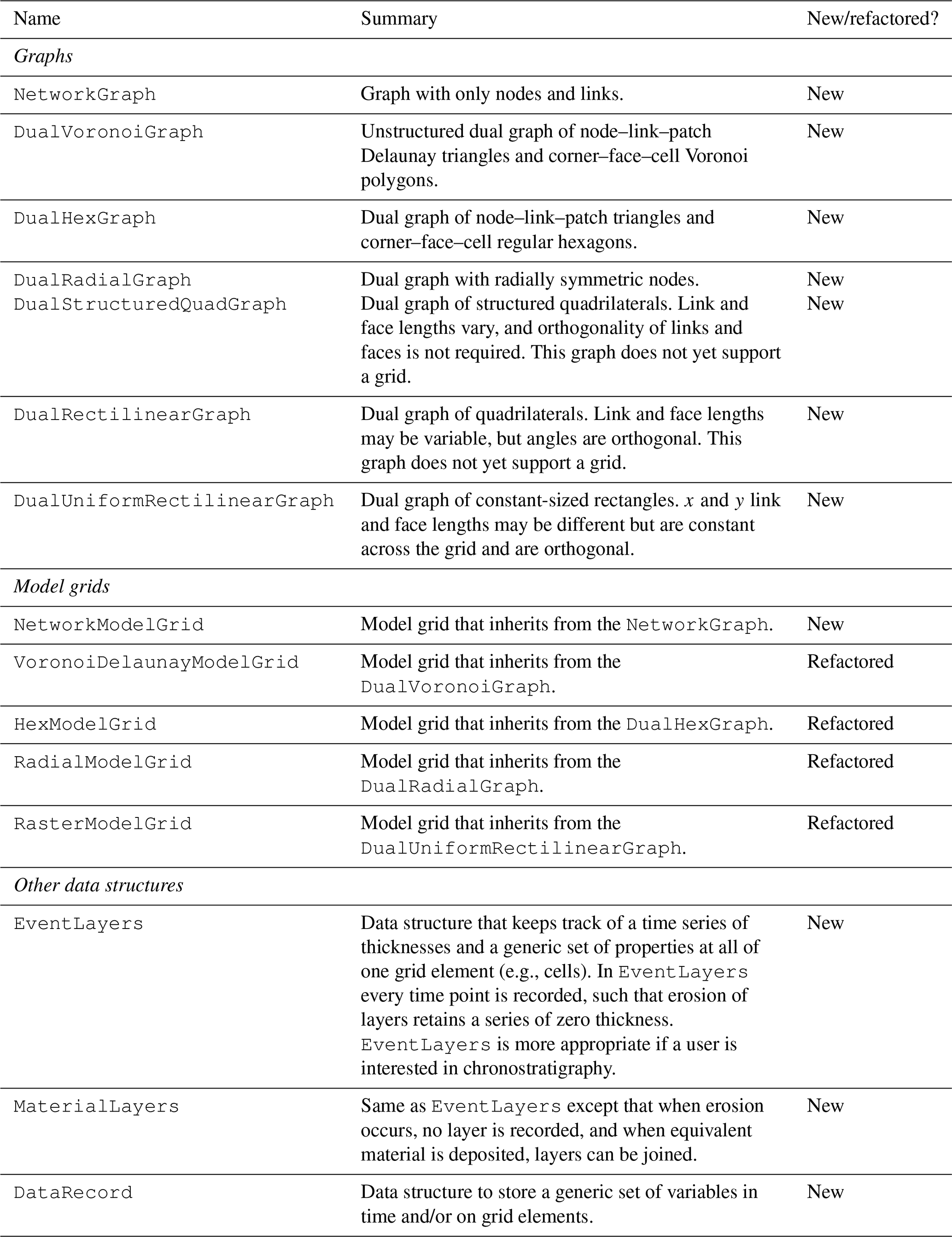
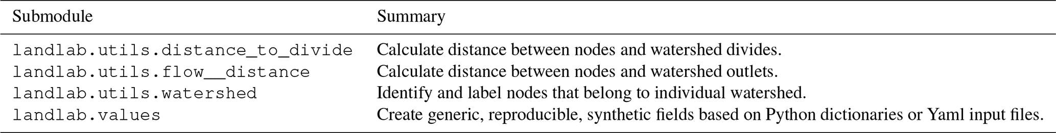
Table 3New components added since Landlab v1.0.
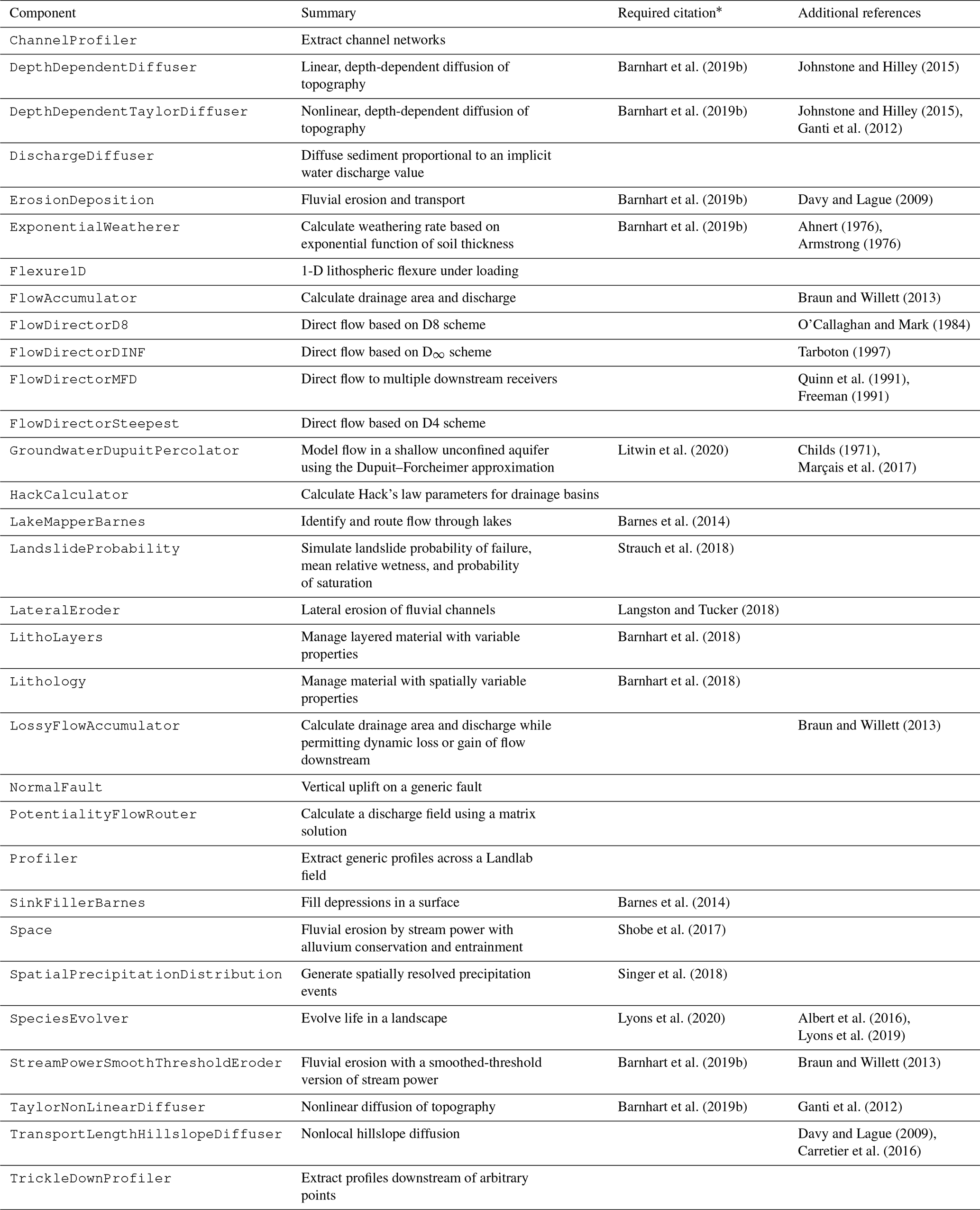
* In addition to Hobley et al. (2017) and this contribution.
Table 4Landlab components in v1.0 (after Hobley et al., 2017, their Table 5).
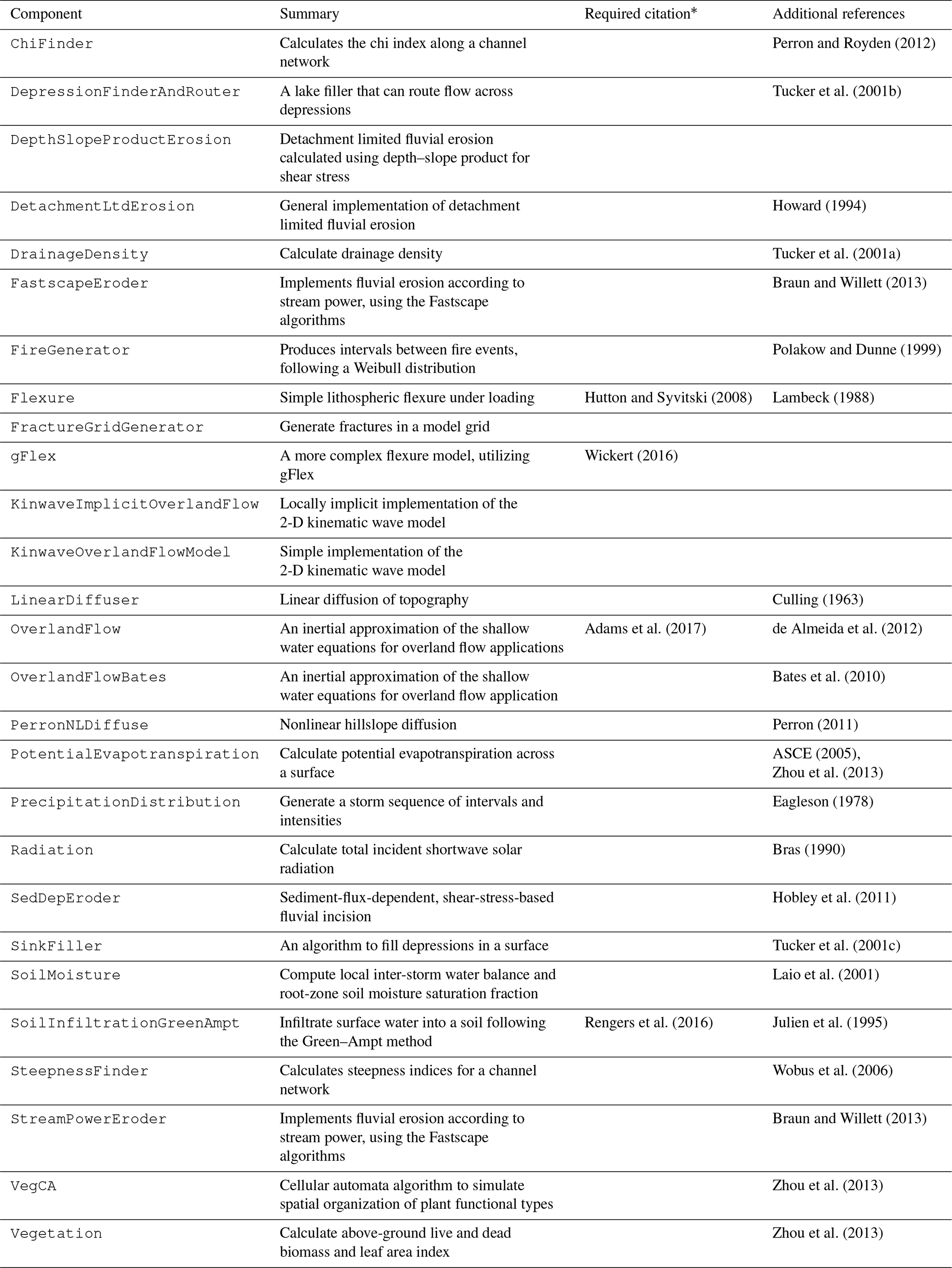
* In addition to Hobley et al. (2017) and this contribution.
This section focuses on the technical details of what has changed between Landlab v1.0 and v2.0. One might glean comparable information from reading the software repositories' change logs. Inclusion of the technical details here is intended to summarize key changes. In addition, where relevant, we describe why changes or improvements were made. This explanation is intended both for current and future users of Landlab as well as for those interested in scientific software development generally.
Changes that broke backward compatibility were required to incorporate some of the new features in Landlab v2.0. This necessitated a new major version. These changes included (i) binding of the boundary condition flags to model grids (Sect. 4.1.3), (ii) a revision to the Component standard interface (Sect. 4.2), (iii) deprecation and removal of certain components and utilities (Sect. 4.3), (iv) dropping Python 2 support (following sunsetting of this version at the end of 2019 by the Python Software Foundation). Additionally, we completely revised the documentation structure (Sect. 4.4). Landlab v2.0 is designed to work with a number of other Python tools for numerical modeling. They are summarized in Sect. 4.5.
4.1 Improvements to the Landlab model grids
Here we highlight three improvements to the Landlab model grid in v2.0.
4.1.1 Grids inherit from graphs
Each Landlab model grid combines a dual graph topology with the ability to store fields at grid elements and keep track of boundary conditions. While the concept of a dual graph is not new in Landlab v2.0, the package architecture has been revised to create a set of graph classes from which the Landlab model grids inherit (Table 1).
The Landlab graphs describe the topology and connectivity of a dual graph of nodes–links–patches/corners–faces–cells and specify the x and y coordinates of the nodes and corners. The package contains support for 1-D and 2-D graphs and for graphs not yet used in Landlab grids (e.g., DualStructuredQuadGraph). It was designed to be reusable by projects external to Landlab. While the graph capabilities do not yet support 3-D graphs, the package was designed with extension to 3-D in mind.
Building the model grids to inherit from the graph data structure results in all model grids containing a complete set of topology-derived attributes (e.g., grid.links_at_node) and attribute naming consistency between model grids. In addition, all of the topology-derived attributes are only created when needed (just-in-time memory allocation) and are cached. This was inconsistently implemented in v1.0 and provides an improvement for memory management and speed.
The graph and model grid data structures are all built on the xarray Python package's Dataset (Hoyer and Hamman, 2016). Using xarray.Dataset provides a number of advantages including improved input and output to the NetCDF format, use of xarray's optimized data structures, and the possibility to take advantage of xarray-compatible parallelization-related tools (e.g., dask; Dask Development Team, 2016; Rocklin, 2015) without breaking backwards compatibility.
4.1.2 Improved treatment of diagonals
The RasterModelGrid can optionally contain an additional grid element called a diagonal, which not only connects nodes but also crosses corners (Fig. 2). Including this grid element violates the assumption of a plane graph because the diagonal elements cross one another. However, use of diagonal elements has a long history in Earth surface dynamics modeling; in order to support historical algorithms (e.g., D8 flow routing, O'Callaghan and Mark, 1984), Landlab's RasterModelGrid contains support for diagonals. This permits studies that cross-compare implementations with and without diagonals (e.g., Shelef and Hilley, 2013).
Landlab v1.0 had a partial implementation of diagonals in which there was no consistent way to refer to the diagonals or the group of linear elements composed of both links and diagonals. In addition, we had an incomplete set of adjacency structures describing diagonals, and we had no mechanism to store values at diagonals on fields. We now consistently call the set of links and diagonals d8s and have implemented adjacency structures and some numerical functions for diagonals and d8s that mirror those for links. Landlab assigns a unique ID to each grid element (see Hobley et al., 2017, their Fig. 4). For example, the nodes are identified with ID numbers from 0 to the number of nodes minus 1, and links are identified with numbers from 0 to the number of links minus 1. The unique IDs assigned to the d8s refer first to the links and then to the diagonals (in this contribution we will use “d8” to refer to the grid element and “D8” to refer to the flow-routing approach).
4.1.3 Boundary condition flags
Landlab v2.0 provides boundary condition status arrays for nodes, links, corners, faces, and, if applicable, diagonals and d8s. Because cells and patches are uniquely associated with their own nodes and corners, we do not supply specific status arrays for those elements. Boundary condition status is indicated by a set of flags that indicate the status (Table 6 indicates flag names; see Hobley et al., 2017, their Sect. 3.1.4 for discussion of boundary conditions). Landlab does not enforce whether a component honors boundary condition flags – the status arrays and flags are provided simply as a convenience to developers. As in v1.0, we enforce internal consistency of boundary conditions across connected grid element types. For example, an update to boundary status at a node will automatically propagate into the connecting links as appropriate and vice versa.
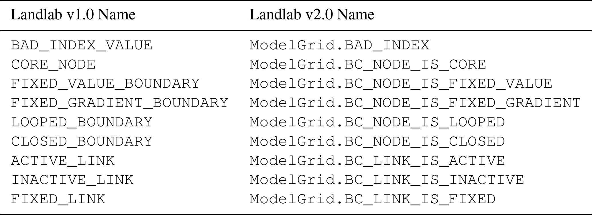
Prior to v2.0, the flags used to indicate node and link status were not formally attached to the model grids and instead existed as separate variables provided by the package. In v2.0 we made boundary condition flags attributes of the grid so that these flags are inseparable from the grids that use them. We also modified the names for clarity (Table 6).
4.2 Updates to the component standard interface
Scientific software and data are much easier to work with when they follows standards. Software tools in particular become much more accessible when they provide a standard interface: a common set of functions that look and act in a similar way across many different elements of the software. Landlab's components use a lightweight interface that is inspired by the CSDMS Basic Model Interface (BMI) (Peckham et al., 2013; Hutton and Piper, 2020a) but which takes advantage of object-oriented features of the Python language, allowing it to be more compact. Landlab also includes built-in functionality that converts any Landlab component into a BMI component, for use in frameworks like the CSDMS Python Modeling Tool (Hutton and Piper, 2020b). In addition to its interface, each Landlab component also encodes metadata in a standardized format; these metadata include, for example, information about the input and output fields of the component.
We made changes to the expectations of component interface, metadata, and code standards based on our experience developing components, supporting community members, and using components in science applications. The enhanced interface standard is designed to improve usability and documentation and to make clearer expectations for contributed components. We have implemented automated tests that ensure existing and contributed components meet this interface standard.
4.2.1 Changes to the component __init__ method
The design of many numerical model programs follows the “initialize-run-finalize” pattern (e.g., Peckham et al., 2013; Hutton and Piper, 2020a). In the BMI, the initialization step is handled by the standard initialize( ) function, and stepwise updating is handled by the update( ) function. For Landlab components, which are implemented as Python objects, the class __init__ method implements initialization, and stepwise updating is normally handled by a method called either run_one_step or update. Hobley et al. (2017, their Sect. 3.3.1) defined the interface for Landlab components with the function signature for instantiation (Component.__init__) and advancing forward (Component.run_one_step). The v1.0 component instantiation interface defined with the function definition as follows: __init__(self, grid, arg1, arg2 …, kwd1 = a, kwd2 = b, kwd3 = c, …, kwds). Here arg1 represents a generic argument, and kwd1 = a represents a generic keyword argument. The kwds was included so that a user could make a single dictionary (or Yaml file) containing all of the keyword arguments for all components used in a model and pass the same dictionary to all components. However, an undesirable side effect of this design was that a slight misspelling of a keyword argument would result in use of the default value with no error raised. To remedy this flaw we revised the instantiation standard to remove the kwds; that is, a user may now only supply the component with input parameters that are explicitly declared in its signature.
In addition we expanded the requirements for component instantiation. These requirements help promote standardization among Landlab components. One new requirement is that components must inherit from the Component base class and call the instantiation method of the base class (super) as part of their instantiation. This ensures that all components take full advantage of the base class functionality and internal checking; for example, the base class will automatically make sure that all of the output fields listed in the header metadata are created, so the component author only needs to ensure that the metadata are present. A related requirement is that by the end of instantiation, all output fields made by the component must exist and have the data type specified by the component metadata. This provides for other components that may check for these fields as input. Finally, a component must raise a sensible error when bad values are provided (for example if an unsupported grid type or unused keyword argument is provided).
4.2.2 Changes to the component run method
The v1.0 component interface defined a run method with a function signature run_one_step(dt, *args, kwds), where dt represents the duration of time the model runs forward, *args represents a generic list of arguments, and kwds represents a generic set of keyword arguments. In practice, we found that many Landlab components were not able to follow this interface standard because it was not flexible enough. For example, some components do not require a dt and thus did not take dt. We also found the presence of *args and kwds in the run_one_step problematic because it complicated wrapping components with a Basic Model Interface (BMI; Peckham et al., 2013; Hutton and Piper, 2020a) for use with the Python Modeling Tool (PyMT; Hutton and Piper, 2020b).
The revised interface balances standardization and flexibility. Components are no longer required to provide a method with the name run_one_step, but if they do not, then an alternative update/execution function must be provided and its usage clearly documented in the header docstring of the component. The new expectation is that if run_one_step is used, it will take either a time duration or nothing. Thus components with a run_one_step method can be easily incorporated into PyMT. Pre-existing components that took arguments or keyword arguments in their run_one_step method have been refactored to either provide those values at instantiation or to use properties, getters, and setters. The terms getter and setter come from object-oriented programming, and they refer to small functions that retrieve the value of (get) or assign a value to (set) a particular variable. Although it might seem odd to create functions to handle such seemingly trivial tasks, the practice has the advantage of enabling defensive programming (e.g., a setter can check for the right data type), allowing a program to create a particular variable only when it is requested (which can save memory), and supporting built-in documentation (in the form of function documentation) for each variable. In Landlab (as in Python practice generally) getters and setters are implemented using the Python @property decorator. Those variables that use getters and setters are considered to be public, meaning that programmers using the component can easily inspect and, if desired, change their values. Other variables are considered private: used only by the component internally and not to be modified (to indicate this, the names of private variables are preceded by an underscore character).
4.2.3 New component metadata standard
For both data and software, standardized metadata promote efficiency, interoperability, and reuse. To that end, each Landlab component includes a set of metadata in the header of the class that defines the component. Our experience with component metadata in Landlab led us to revise its design for version 2.0.
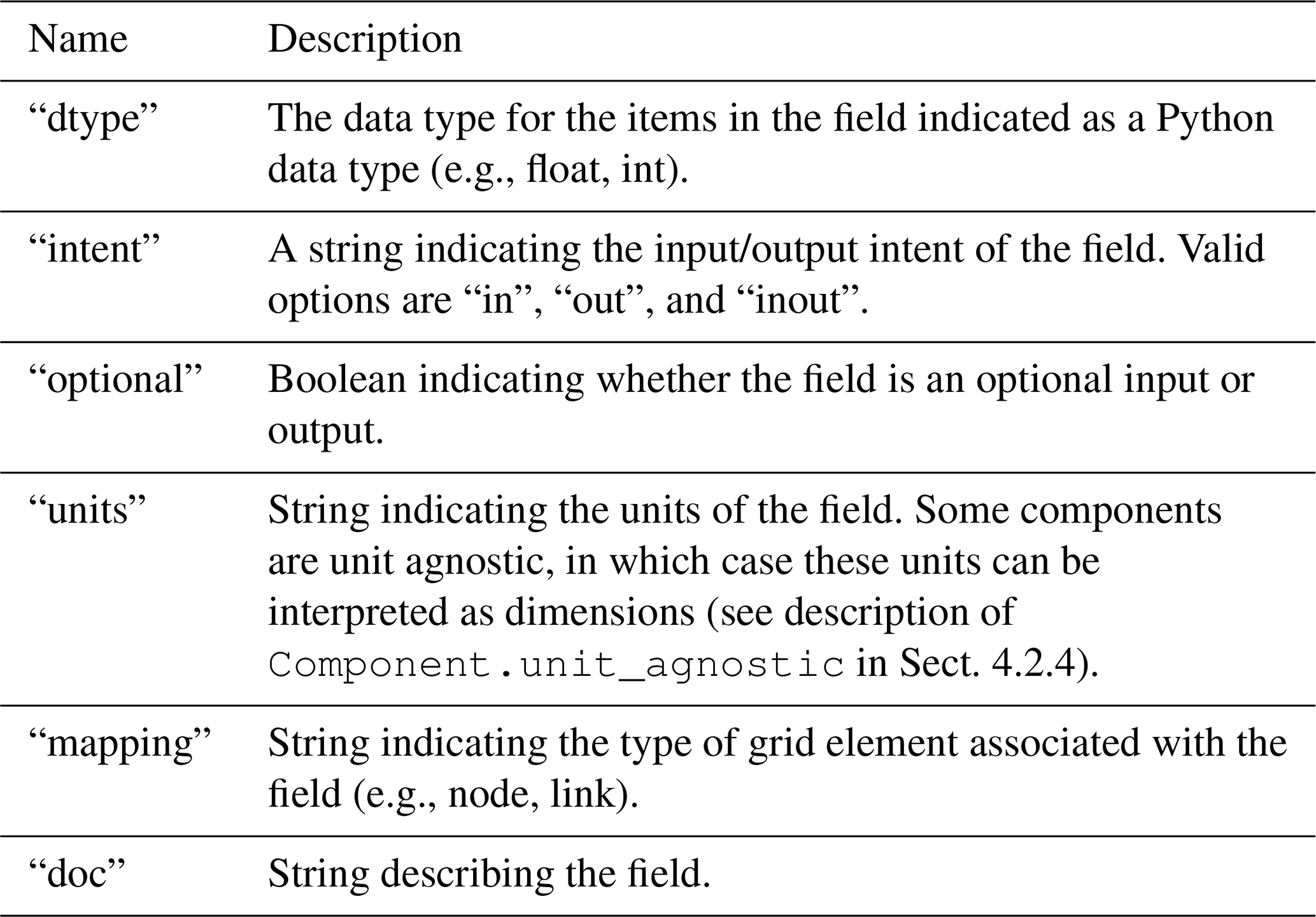
The metadata section of a Landlab component describes its input fields, output fields, field units, the type of grid element associated with each field, and a long-format description of the field. Metadata are now organized into a single Python dictionary, which has a key-value pair for each field used by the component. The new data structure makes it easier to test for completeness and consistency across components. Each key is a string indicating the field name. The associated value is itself a dictionary that has a standard, required set of keys (Table 7).
4.2.4 Additional component content requirements and recommendations
Here we highlight the few remaining component requirements and recommendations. The use of must indicates a requirement, while the use of may or should indicates a recommendation.
-
All public attributes must be documented properties of the
Componentclass; that is, they have the@propertystandard Python decorator. This ensures that other users are able to identify what each public attribute is and prevents variable modification unless the developer explicitly permits it. This change has little impact on developers time because a developer may elect to use only private attributes. -
If a developer envisions that the public attribute of a component may be modified, they must create a
setterfor it. This provides a place for a component author to write checks that ensure a user cannot incorrectly assign invalid component attributes. -
Field names shared between multiple components must use a consistent definition and dimensions. Some components require parameters and fields to use a particular set of units, while others are unit agnostic. This is flagged in the component attribute
Component.unit_agnostic. It is up to the user to ensure that an application uses consistent units across all fields, components, and input parameters. -
Arguments and keyword arguments should start with lowercase letters.
-
The grid should be the only argument to the component __
init__. All other inputs are provided as keyword arguments. -
Keyword arguments should have reasonable default values so that all keywords are truly optional.
-
The main method of a component (either
run_one_stepor a custom-designed update/execution function) should return either nothing, the grid, or a single calculated value.
4.3 Removed or modified components and utilities
Several obsolete components and utilities have been removed from Landlab v2.0. Other components were substantially modified. Here we describe these changes.
-
The
FlowRoutercomponent, which did D8 and D4/steepest descent flow routing and accumulation, was removed and replaced with theFlowAccumulatorand a family ofFlowDirectorcomponents. This change provides greater flexibility in options for flow-routing algorithms (e.g., multiple flow directions, D∞). -
The routing-based surface-water erosion components (such as
StreamPowerEroder) now use a single consistent method for handling the input runoff rate. The keyword argumentrunoff_rateto theFlowAccumulatorcan now specify a float, array, or field name indicating the runoff rate. This is then accumulated to create the fieldsurface__water_discharge, which can be used by components that model surface-water erosion. -
The
ModelParameterDictionarywas removed because it represents an old-style input file that has been superseded by the Yaml format. -
A new
ChannelProfilercomponent replaces the previous channel-profiling submodule (landlab.plot.channel_profile). -
The
noclobberkeyword argument for field creation was changed toclobberbecause the original name required double negatives and was not intuitive.noclobber=Falseis equivalent toclobber=True. -
The ability to pass an array of flooded nodes to the
run_one_stepmethod in surface-water erosion components was removed and replaced with a keyword argument to __init__ callederode_flooded_nodes.
4.4 Reorganization of the Landlab documentation
The Landlab online documentation is now consolidated onto a single Sphinx-based platform (https://landlab.readthedocs.io/, last access: 12 May 2020). Consolidating the documentation onto a single platform with a consistent interface reduces duplication of information, improves consistency, and permits comprehensive searches. The site design is similar to that of widely used scientific Python packages and was modeled after that of pandas (McKinney, 2010). The revised documentation pages include installation instructions, a user guide (including tutorials), a guide for developers, and an API reference that contains formatted versions of inline documentation within the source code. The documentation source is written in reStructuredText format, and the source files are provided as part of the Landlab package.
4.5 Packages built to work with Landlab
Landlab was designed as a generic, extensible modeling framework for Earth surface dynamics. Because Landlab exposes a BMI (Hutton and Piper, 2020a), it is compatible with the PyMT package (Hutton and Piper, 2020b) – a Python package that supports running and coupling models that expose a BMI. PyMT provides access to a suite of models written in multiple languages (e.g., Python, Fortran, C) and a standard interface for initializing and running.
In addition, two packages have been built using Landlab to support applications in sensitivity analysis, calibration, validation, and multimodel comparison (see Barnhart et al., 2020a, b, c, for example applications). First, terrainbento is a Python package for multimodel analysis that provides an extensible set of 27 Landlab-built models for long-term drainage basin and landform evolution, along with general classes for handling boundary conditions through an input-file format (Barnhart et al., 2019b). Second, umami is used to calculate model–data comparison metrics for observed and simulated topography (Barnhart et al., 2019a).
Citation of scientific software is an outstanding challenge (e.g., Niemeyer et al., 2016). Scientific software is cited less frequently than it is used (e.g., Pan et al., 2015). Indicating a recommended citation for use of Landlab is additionally challenging because, depending on the portion of Landlab used, the set of citations required may vary. We describe our recommendations for which citations to use and present a tool within Landlab to improve citation discoverability.
Any time any part of Landlab is used, Hobley et al. (2017) should be cited; if the version used is >1.0, then this contribution should be additionally cited. These two citations acknowledge the development of the Landlab package itself. We also recommend that authors state the specific version of Landlab used (the version can be found by evaluating landlab.__version__).
Each application of Landlab may use a different set of components, each with a different citation for the software itself and general set of theory references (Tables 3 and 4). Additionally, some parts of Landlab may internally use others; thus a user may not easily be able to assess the entire set of elements of Landlab their application has used and what to cite for each part.
This challenge is not new. For example, it is faced by the scipy package, which addresses it by providing a core-package citation – Virtanen et al. (2019) – and indicating that users should look to the reference section of the documentation for additional citations. Similarly, the codes distributed through the Computational Infrastructure for Geodynamics (CIG) have a citation builder that distinguishes between citations specific to the software implementation, primary citations describing the code development and numerical methods, and secondary citations that pertain to parts of the code a user may or may not have used (Kellogg et al., 2018). This example from CIG highlights a further challenge: a component may have one or more citations for each of the following categories: (i) the theory behind the implemented idea, (ii) a description of the software implementation itself, (iii) any specialized algorithms developed for the implementation, and (iv) the first reported use of the software in a publication.
Should one of these or all of these be the recommended and/or required citations for a given software component? We do not think it is our role to decide which citations, if any, a component author indicates as recommended or required. Additionally, it is not our place – as the software developers behind Landlab – to determine which citations best represent the theory behind an implementation. Instead we provide two places for a component author to indicate what they think the minimum required citations are as follows: a component attribute called Component.cite_as which lists required citations for a given component and a section in the component docstring that provides the broader reference context. These two categories are reflected by the two citation columns in Tables 3 and 4. Clearly, a component developer has the authority to decide exactly what to put in either of these locations.
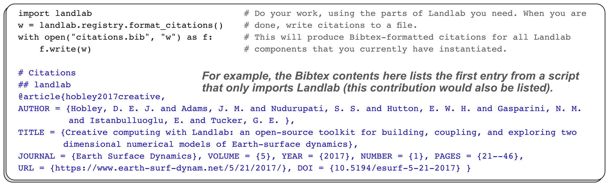
To aid discoverability of citations, we have created the Landlab citation registry, a tool that compiles citation-related metadata for the specific set of Landlab components used in an application (Listing 3). The citation registry compiles citation information for all components currently instantiated in a Python session by automatically interrogating their cite_as properties.
In this section we highlight several lessons about software development we have learned in the processes of supporting and improving Landlab v1.0 to its current v2.0 state and working with the growing community of users.
We reflect on these lessons because the production of research software is itself research, and there are many aspects of scientific software which are distinct from other software, notably that (i) the development lifecycle includes additional stages because the methods used to implement a piece of software may not exist at the outset of a project, (ii) requirements evolve because they are part of the research, and (iii) the state of the scientific field may be complex and evolving (e.g., Carver et al., 2016).
6.1 Value of testing
The development of docstring and unit tests within Landlab was motivated by following software development best practices (e.g., Wilson et al., 2014, 2017). That is, our focus was on ensuring that the package behaves as described and, where an analytical solution exists, that Landlab correctly solves it. While using a testing suite is standard in many software development contexts, it is relatively uncommon in scientific software development (e.g., Prabhu et al., 2011). Tests do not ensure that elements of the Landlab software represent the truth or guarantee that a model is appropriate for a specific application; in other words, Landlab cannot and does not attempt to validate (sensu Schlesinger et al., 1979) the assumptions of its components. Instead, the tests verify (Schlesinger et al., 1979) that the software is behaving as expected and that numerical methods are solving stated equations reliably. Through coupled use of an automatic testing suite and continuous integration we ensure that changes to the code base do not break existing tests.
The process of developing Landlab, working with its user community, and revising it to v2.0 illustrated another, obvious in retrospect, benefit of the tests: developing a set of tests for the package interface and numerical behavior make it possible to refactor. Without these tests, it would have been much more difficult to implement beneficial revisions (such as refactoring the model grid to derive from the graph-based class).
Writing effective unit tests that ensure Landlab components reliably solve their equations under a variety of initial and boundary conditions is not a trivial task. When a set of equations that a component solves have an analytical solution then the numerics of a component can be verified based on the ability to reproduce such a relationship (e.g., stream power erosion produces a known slope-area relationship, Willgoose et al., 1991). When such analytical predictions do not exist—as is often the case—a more detailed analysis of the equations must be performed in order to create a full verification test. Even in the absence of such analytical solutions, however, many existing components have made headway during development simply by testing for mass balance and timestep consistency, and the value of such simplifications should not be ignored.
In contrast, it is much easier to design and implement tests for the Landlab interface (e.g., when an invalid value is passed to a component, is the correct type of error raised). In general, designing a thorough set of tests is a learned skill that requires thinking through many edge cases of model behavior.
6.2 Collaborative development of research software requires many skills
Scientific software development requires distinct skills. Based on working with community user-developers and onboarding new members of the core development team, we describe the set of skills that are needed to interact with a project like Landlab as a user-developer. Our intention here is to document a concrete example so that efforts to create scientific software development curricula can be based on use-cases. In the case of Landlab, the skills required to contribute to the project include:
-
Python programming, including functions, classes, and basic package organization.
-
Fundamental elements of version control using git (branching, commits).
-
GitHub for collaboration (issues trackers, merging, pull requests, managing forks, code reviews).
-
Package dependency management (currently implemented with conda environments).
-
Conceptual design and practical implementation of unit tests.
-
reStructuredText syntax for creating documentation.
In addition, there are a number of skills that not all user-developers need but are necessary to have within the project team in order to maintain continuous integration, documentation, building binaries, and distributing (e.g., sphinx, configuring and debugging continuous integration platforms).
The importance of these skills is highlighted in the context of technical debt, or the cost of implementing a fast and easy solution now, as opposed to a better approach that may take longer. For example, we have found that it is much easier to create content than to make it accessible (this observation motivated the restructuring of the documentation described in Sect. 4.4). It is also easier to write code than to write thorough and effective tests for it, yet omitting tests greatly increases the risk of serious bugs, which can invalidate the research that the software is meant to facilitate.
6.3 Balancing the burden on developers and users
Open-source software (scientific or otherwise) commonly has many more users than developers or user-developers (e.g., numpy). Under those circumstances, moderate investments in developer time are justified to make use faster or more intuitive for users. However, Landlab is a case with slightly different dynamics, which are worth reflecting on. Landlab is an example of a niche scientific software package with a relatively small development community. Here we reflect on some of the development dynamics of this type of scientific software and the relative burdens for use on developers and users.
Our goal is to create an extensible software package that solves a variety of Earth surface dynamics problems and is accessible to undergraduates and active researchers and to support community members in contributing to the code (transitioning from users to user-developers). Effectively serving the community requires a balance between minimizing technical debt (by enforcing standards within the code base), while also making development and contribution accessible to inexperienced but motivated community members.
One aspect of our approach, inspired by experience working with community members, is to be flexible with the software engineering and interface standards. This includes relaxing standards when necessary. For example, while a strict interface standard for components would likely reduce technical debt, our experience is that such rigidity would raise a substantial barrier to community contribution. This means that we need to strike a balance in our design principles between standardization and flexibility (e.g., relaxing the standard for the run_one_step method described in Sect. 4.2).
Second, we embrace the idea that good is better than not at all. That is, some tests are better than none, meaningful tests are better than non-meaningful ones, and bare-bones documentation is better than none. We find that documentation improves the most when users try to use it, find that it is insufficient or unclear, and interact with developers through the online and open GitHub Issues forum. Users and developers then together revise the text. Because the development team is small and supported primarily by grants, we rely on users to indicate where improvements must be made.
We highly encourage all contributions to Landlab. The package is designed as an extensible piece of community software, and we look forward to it growing to meet community needs. Common ways that an interested individual might get started include the following: identifying or making improvements to the documentation and example notebooks, finding and fixing bugs, and describing and creating desired features – such as new components. For information about how to get started, including source code and prepackaged binary installation (via PyPI or conda-forge), visit the website at https://landlab.readthedocs.io/ (last access: 12 May 2020).
Landlab v2.0 provides the community with a robust and extensible package for modeling Earth surface dynamics. It is distributed as source code and as prepackaged binaries for Linux, MacOS, and Windows. An extensive set of unit tests ensure reliability of the code base. This version provides substantial improvements over v1.0 including (i) a revised set of model grid classes, (ii) updates to the component interface, (iii) 31 new components, (iv) expanded and consolidated documentation, and (v) a tool for identifying appropriate citations. The backward-compatibility-breaking changes made in Landlab v2.0 reflect changes necessary based on use and development of the package. The modular design of Landlab means that developers only need to create the new piece they need, and researchers can mix and match components to create a desired model. As a tested, version-controlled, and documented software package, Landlab reduces barriers to computational modeling and supports reproducible research.
The v2.0 version of the software is provided as a supplement to this contribution and is archived with Zenodo (Hutton et al., 2020).
KRB and EWHH led the design and v2.0 refactoring of the Landlab package with input from all coauthors. KRB wrote the original draft of the paper, with input from all coauthors. All authors edited the paper. KRB, EWHH, GET, NMG, DEJH, NJL, MM, SSN, and JMA contributed to the Landlab code base. All authors designed and taught short courses which provided usability testing and resulted in critical improvements to package architecture and documentation. CB expanded accessibility of Landlab using advanced cyberinfrastructure by leading integration of Landlab with the HydroShare platform. GET, NMG, EI, and EWHH conceptualized Landlab and created its prototype. GET, NMG, EI, and DEJH acquired the core funding to support Landlab, with additional funding acquired by KRB, CB, and NJL.
The authors declare that they have no conflict of interest.
Funding sources for Landlab are acknowledged in the next section. In addition, we recognize support and guidance from the Community Surface Dynamics Modeling System. We thank Tristan Salles and Wolfgang Schwanghart for thoughtful reviews, and Simon Mudd for serving as handling editor. Tony Castronova and the Consortium of Universities for the Advancement of Hydrologic Science, Inc. support use of Landlab on the HydroShare Platform (NSF EAR 1338606). Landlab Group members on HydroShare have freely shared research, data, training, and teaching resources with Landlab and HydroShare communities. Landlab relies on free open-source package builds from TravisCI and Appveyor for our continuous integration. Our documentation is hosted for free by ReadTheDocs.
Landlab would not exist without decades of open-source software development. In this spirit, we thank all community members who have asked questions, made issues, commented on documentation that did not make sense, and contributed code to the package. Below we list the results of our best efforts to compile all non-author community contributors to the Landlab package source code. The are as follows (in alphabetical order): Guiseppe Cippolla, Jon Czuba, Vanessa Gabel, Rachel Glade, Jenny Knuth, Abby Langston, David Litwin, Amanda Manaster, Allison Pfeiffer, Francis Rengers, Charlie Shobe, and Rhonda Strauch.
This research has been supported by the US National Science Foundation (grant nos. 1147454, 1450409, 1147519, 1450338, 1148305, 1450412, 1246761, 1725774, 1902600, 1226297, and 1831623), the Marie Curie/Sêr Cymru II Cofund Research Fellowship (grant no. 663830-CU-035), a Software Sustainability Institute Fellowship, and a Tulane University Oliver Fund Scholar Award.
This paper was edited by Simon Mudd and reviewed by Tristan Salles and Wolfgang Schwanghart.
Adams, J. M., Gasparini, N. M., Hobley, D. E. J., Tucker, G. E., Hutton, E. W. H., Nudurupati, S. S., and Istanbulluoglu, E.: The Landlab v1.0 OverlandFlow component: a Python tool for computing shallow-water flow across watersheds, Geosci. Model Dev., 10, 1645–1663, https://doi.org/10.5194/gmd-10-1645-2017, 2017. a
Adorf, C. S., Ramasubramani, V., Anderson, J. A., and Glotzer, S. C.: How to Professionally Develop Reusable Scientific Software – And When Not To, Comput. Sci. Eng., 21, 66–79, https://doi.org/10.1109/mcse.2018.2882355, 2019. a
Ahnert, F.: Brief description of a comprehensive three-dimensional process-response model of landform development, Z. Geomorphol. Suppl. Band, 25, 29–49, 1976. a
Albert, J. S., Schoolmaster Jr., D. R., Tagliacollo, V., and Duke-Sylvester, S. M.: Barrier Displacement on a Neutral Landscape: Toward a Theory of Continental Biogeography, System. Biol., 66, 167–182, https://doi.org/10.1093/sysbio/syw080, 2016. a
Armstrong, A. C.: A three dimensional simulation of slope forms, Z. Geomorphol., 25, 20–28, 1976. a
ASCE: The ASCE Standardized Reference Evapotranspiration Equation, in: Standardization of Reference Evapotranspiration Task Committee Final Report, edited by: Allen, R. G., Walter, I. A., Elliot, R. L., Howell, T. A., Itenfisu, D., Jensen, M. E., and Snyder, R. L., Technical Committee report to the Environmental and Water Resources Institute of the American Society of Civil Engineers from the Task Committee on Standardization of Reference Evapotranspiration, Reston, VA, USA, 2005. a
Bandaragoda, C., Castronova, A., Istanbulluoglu, E., Strauch, R., Nudurupati, S., Phuong, J., Adams, J., Gasparini, N., Barnhart, K. R., Hutton, E., Hobley, D., Lyons, N. J., Tucker, G. E., Tarboton, D. G., Idaszak, R., and Wang, S.-W.: Enabling Collaborative Numerical Modeling in Earth Sciences using Knowledge Infrastructure, Environ. Model. Softw., 120, 104424, https://doi.org/10.1016/j.envsoft.2019.03.020, 2019. a
Barnes, R., Lehman, C., and Mulla, D.: Priority-flood: An optimal depression-filling and watershed-labeling algorithm for digital elevation models, Comput. Geosci., 62, 117–127, https://doi.org/10.1016/j.cageo.2013.04.024, 2014. a, b
Barnhart, K. R., Hutton, E., Gasparini, N., and Tucker, G.: Lithology: A Landlab submodule for spatially variable rock properties, J. Open Sour. Softw., 3, 979, https://doi.org/10.21105/joss.00979, 2018. a, b
Barnhart, K. R., Hutton, E., and Tucker, G.: umami: A Python package for Earth surface dynamics objective function construction, J. Open Sour. Softw., 4, 1776, https://doi.org/10.21105/joss.01776, 2019a. a
Barnhart, K. R., Glade, R. C., Shobe, C. M., and Tucker, G. E.: Terrainbento 1.0: a Python package for multi-model analysis in long-term drainage basin evolution, Geosci. Model Dev., 12, 1267–1297, https://doi.org/10.5194/gmd-12-1267-2019, 2019b. a, b, c, d, e, f, g
Barnhart, K. R., Tucker, G. E., Doty, S., Shobe, C. M., Glade, R. C., Rossi, M. W., and Hill, M. C.: Inverting topography for landscape evolution model process representation: Part 1. Conceptualization and sensitivity analysis, J. Geophys. Res.-Earth, 125, e2018JF004961, https://doi.org/10.1029/2018JF004961, 2020a. a
Barnhart, K. R., Tucker, G. E., Doty, S., Shobe, C. M., Glade, R. C., Rossi, M. W., and Hill, M. C.: Inverting topography for landscape evolution model process representation: Part 2. Calibration and validation, J. Geophys. Res.-Earth, 125, e2018JF004963, https://doi.org/10.1029/2018JF004963, 2020b. a
Barnhart, K. R., Tucker, G. E., Doty, S., Shobe, C. M., Glade, R. C., Rossi, M. W., and Hill, M. C.: Inverting topography for landscape evolution model process representation: Part 3. Determining parameter ranges for select mature geomorphic transport laws and connecting changes in fluvial erodibility to changes in climate, J. Geophys. Res.-Earth, e2019JF005287, https://doi.org/10.1029/2019JF005287, 2020c. a
Bates, P. D., Horritt, M. S., and Fewtrell, T. J.: A simple inertial formulation of the shallow water equations for efficient two-dimensional flood inundation modelling, J. Hydrol., 387, 33–45, https://doi.org/10.1016/j.jhydrol.2010.03.027, 2010. a
Bras, R.: Hydrology: An introduction to hydrologic science, Addison-Wesley, Reading, MA, USA, 1990. a
Braun, J. and Willett, S. D.: A very efficient O(n), implicit and parallel method to solve the stream power equation governing fluvial incision and landscape evolution, Geomorphology, 180-181, 170–179, https://doi.org/10.1016/j.geomorph.2012.10.008, 2013. a, b, c, d, e
Carretier, S., Martinod, P., Reich, M., and Godderis, Y.: Modelling sediment clasts transport during landscape evolution, Earth Surf. Dynam., 4, 237–251, https://doi.org/10.5194/esurf-4-237-2016, 2016. a
Carver, J. C., Hong, N. P. C., and Thiruvathukal, G. K.: Software engineering for science, CRC Press, Boca Raton, FL, USA, 2016. a
Chen, X., Dallmeier-Tiessen, S., Dasler, R., Feger, S., Fokianos, P., Gonzalez, J. B., Hirvonsalo, H., Kousidis, D., Lavasa, A., Mele, S., Rodriguez, D. R., Šimko, T., Smith, T., Trisovic, A., Trzcinska, A., Tsanaktsidis, I., Zimmermann, M., Cranmer, K., Heinrich, L., Watts, G., Hildreth, M., Iglesias, L. L., Lassila-Perini, K., and Neubert, S.: Open is not enough, Nat. Phys., 15, 113–119, https://doi.org/10.1038/s41567-018-0342-2, 2018. a
Childs, E. C.: Drainage of Groundwater Resting on a Sloping Bed, Water Resour. Res., 7, 1256–1263, https://doi.org/10.1029/wr007i005p01256, 1971. a
Culling, W. E. H.: Soil Creep and the Development of Hillside Slopes, J. Geol., 71, 127–161, https://doi.org/10.1086/626891, 1963. a
Dask Development Team: Dask: Library for dynamic task scheduling, available at: https://dask.org (last access: 12 May 2020), 2016. a, b
Davy, P. and Lague, D.: Fluvial erosion/transport equation of landscape evolution models revisited, J. Geophys. Res., 114, F03007, https://doi.org/10.1029/2008jf001146, 2009. a, b
de Almeida, G. A. M., Bates, P., Freer, J. E., and Souvignet, M.: Improving the stability of a simple formulation of the shallow water equations for 2-D flood modeling, Water Resour. Res., 48, W05528, https://doi.org/10.1029/2011wr011570, 2012. a
Eagleson, P. S.: Climate, soil, and vegetation: 2. The distribution of annual precipitation derived from observed storm sequences, Water Resour. Res., 14, 713–721, https://doi.org/10.1029/wr014i005p00713, 1978. a
Freeman, T. G.: Calculating catchment area with divergent flow based on a regular grid, Comput. Geosci., 17, 413–422, https://doi.org/10.1016/0098-3004(91)90048-i, 1991. a
Ganti, V., Passalacqua, P., and Foufoula-Georgiou, E.: A sub-grid scale closure for nonlinear hillslope sediment transport models, J. Geophys. Res.-Earth, 117, F02012, https://doi.org/10.1029/2011jf002181, 2012. a, b
Hobley, D. E. J., Sinclair, H. D., Mudd, S. M., and Cowie, P. A.: Field calibration of sediment flux dependent river incision, J. Geophys. Res., 116, F04017, https://doi.org/10.1029/2010jf001935, 2011. a
Hobley, D. E. J., Adams, J. M., Nudurupati, S. S., Hutton, E. W. H., Gasparini, N. M., Istanbulluoglu, E., and Tucker, G. E.: Creative computing with Landlab: an open-source toolkit for building, coupling, and exploring two-dimensional numerical models of Earth-surface dynamics, Earth Surf. Dynam., 5, 21–46, https://doi.org/10.5194/esurf-5-21-2017, 2017. a, b, c, d, e, f, g, h, i, j, k
Howard, A. D.: A detachment-limited model of drainage basin evolution, Water Resour. Res., 30, 2261–2285, https://doi.org/10.1029/94wr00757, 1994. a
Hoyer, S. and Hamman, J.: xarray: N-D labeled Arrays and Datasets in Python, J. Open Res. Softw., 5, 10, https://doi.org/10.5334/jors.148, 2016. a, b
Hunter, J. D.: Matplotlib: A 2D Graphics Environment, Comput. Sci. Eng., 9, 90–95, https://doi.org/10.1109/mcse.2007.55, 2007. a
Hutton, E. W. H. and Piper, M.: csdms/bmi-python: v2.0, zenodo, https://doi.org/10.5281/zenodo.3647556, 2020a. a, b, c, d, e
Hutton, E. W. H. and Piper, M.: csdms/pymt: The Python Modeling Toolkit, zenodo, https://doi.org/10.5281/zenodo.3644240, 2020b. a, b, c
Hutton, E. W. H. and Syvitski, J. P.: Sedflux 2.0: An advanced process-response model that generates three-dimensional stratigraphy, Comput. Geosci., 34, 1319–1337, https://doi.org/10.1016/j.cageo.2008.02.013, 2008. a
Hutton, E. W. H., Barnhart, K. R., Hobley, D. E. J., Tucker, G. E., Nudurupati, S. S., Adams, J. M., Gasparini, N. M., Shobe, C. M., Strauch, R., Knuth, J., Mouchene, M., Lyons, N., Litwin, D., Glade, R., Cipolla, G., Manaster, A., Langston, A., Thyng, K., and Rengers, F.: landlab/landlab: Mrs. Weasley, zenodo, https://doi.org/10.5281/zenodo.3776837, 2020. a
Hwang, L., Fish, A., Soito, L., Smith, M., and Kellogg, L. H.: Software and the scientist: Coding and citation practices in geodynamics, Earth Space Sci., 4, 670–680, https://doi.org/10.1002/2016EA000225, 2017. a
Johnstone, S. A. and Hilley, G. E.: Lithologic control on the form of soil-mantled hillslopes, Geology, 43, 83–86, https://doi.org/10.1130/g36052.1, 2015. a, b
Julien, P. Y., Saghafian, B., and Ogden, F. L.: Raster-based hydrologic modeling of spatially-varied surface runoff, J. Am. Water Resour. Assoc., 31, 523–536, https://doi.org/10.1111/j.1752-1688.1995.tb04039.x, 1995. a
Kellogg, L. H., Hwang, L. J., Gassmoller, R., Bangerth, W., and Heister, T.: The Role of Scientific Communities in Creating Reusable Software: Lessons From Geophysics, Comput. Sci. Eng., 21, 25–35, https://doi.org/10.1109/mcse.2018.2883326, 2018. a
Kluyver, T., Ragan-Kelley, B., Pérez, F., Granger, B., Bussonnier, M., Frederic, J., Kelley, K., Hamrick, J., Grout, J., Corlay, S., Ivanov, P., Avila, D., Abdalla, S., and Willing, C.: Jupyter Notebooks – a publishing format for reproducible computational workflows, in: Positioning and Power in Academic Publishing: Players, Agents and Agendas, edited by: Loizides, F. and Schmidt, B., IOS Press, Amsterdam, the Netherlands, 87–90, 2016. a
Krekel, H., Oliveira, B., Pfannschmidt, R., Bruynooghe, F., Laugher, B., and Bruhin, F.: pytest 5.3.2, available at: https://github.com/pytest-dev/pytest (last access: 12 May 2020), 2004. a
Lai, J. and Anders, A. M.: Modeled Postglacial Landscape Evolution at the Southern Margin of the Laurentide Ice Sheet: Hydrological Connection of Uplands Controls the Pace and Style of Fluvial Network Expansion, J. Geophys. Res.-Earth, 123, 967–984, https://doi.org/10.1029/2017JF004509, 2018. a
Laio, F., Porporato, A., Ridolfi, L., and Rodriguez-Iturbe, I.: Plants in water-controlled ecosystems: active role in hydrologic processes and response to water stress II. Probabilistic soil moisture dynamics, Adv. Water Resour., 24, 707–723, https://doi.org/10.1016/s0309-1708(01)00005-7, 2001. a
Lambeck, K.: Geophysical Geodesy: The Slow Deformations of the Earth, Clarendon, Oxford, 1988. a
Langston, A. L. and Tucker, G. E.: Developing and exploring a theory for the lateral erosion of bedrock channels for use in landscape evolution models, Earth Surf. Dynami., 6, 1–27, https://doi.org/10.5194/esurf-6-1-2018, 2018. a
Litwin, D., Tucker, G., Barnhart, K., and Harman, C.: GroundwaterDupuitPercolator: A Landlab component for groundwater flow, J. Open Sour. Softw., 5, 1935, https://doi.org/10.21105/joss.01935, 2020. a
Lyons, N. J., Val, P., Albert, J. S., Willenbring, J. K., and Gasparini, N. M.: Topographic controls on divide migration, stream capture, and diversification in riverine life, Earth Surf. Dynam. Discuss., https://doi.org/10.5194/esurf-2019-55, in review, 2019. a
Lyons, N. J., Albert, J. S., and Gasparini, N. M.: SpeciesEvolver: A Landlab component to evolve life in simulated landscapes, J. Open Sour. Softw., 5, 2066, https://doi.org/10.21105/joss.02066, 2020. a
Mandli, K. T., Ahmadia, A. J., Berger, M., Calhoun, D., George, D. L., Hadjimichael, Y., Ketcheson, D. I., Lemoine, G. I., and LeVeque, R. J.: Clawpack: building an open source ecosystem for solving hyperbolic PDEs, PeerJ. Comp. Sci., 2, e68, https://doi.org/10.7717/peerj-cs.68, 2016. a
Marçais, J., Dreuzy, J.-R. D., and Erhel, J.: Dynamic coupling of subsurface and seepage flows solved within a regularized partition formulation, Adv. Water Resour., 109, 94–105, https://doi.org/10.1016/j.advwatres.2017.09.008, 2017. a
McKinney, W.: Data Structures for Statistical Computing in Python, edited by: van der Walt, S. and Millman, J., Proceedings of the 9th Python in Science Conference, Austin, TX, USA, 51–56, 2010. a, b
Niemeyer, K. E., Smith, A. M., and Katz, D. S.: The Challenge and Promise of Software Citation for Credit, Identification, Discovery, and Reuse, J. Data Inform. Qual., 7, 5, https://doi.org/10.1145/2968452, 2016. a
O'Callaghan, J. F. and Mark, D. M.: The extraction of drainage networks from digital elevation data, Computer Vis. Graph. Image Proc., 28, 323–344, https://doi.org/10.1016/s0734-189x(84)80011-0, 1984. a, b
Pan, X., Yan, E., Wang, Q., and Hua, W.: Assessing the impact of software on science: A bootstrapped learning of software entities in full-text papers, J. Informetr., 9, 860–871, https://doi.org/10.1016/j.joi.2015.07.012, 2015. a
Peckham, S. D., Hutton, E. W. H., and Norris, B.: A component-based approach to integrated modeling in the geosciences The design of CSDMS, Comput. Geosci., 53, 3–12, https://doi.org/10.1016/j.cageo.2012.04.002, 2013. a, b, c, d, e
Pérez, F. and Granger, B. E.: IPython: A System for Interactive Scientific Computing, Comput. Sci. Eng., 9, 21–29, https://doi.org/10.1109/mcse.2007.53, 2007. a
Perron, J. T.: Numerical methods for nonlinear hillslope transport laws, J. Geophys. Res., 116, 23–13, https://doi.org/10.1029/2010jf001801, 2011. a
Perron, J. T. and Royden, L.: An integral approach to bedrock river profile analysis, Earth Surf. Proc. Land., 38, 570–576, https://doi.org/10.1002/esp.3302, 2012. a
Poisot, T.: Best publishing practices to improve user confidence in scientific software, Idea. Ecol. Evol., 8, 50–54, https://doi.org/10.4033/iee.2015.8.8.f, 2015. a
Polakow, D. A. and Dunne, T. T.: Modelling fire-return interval T: stochasticity and censoring in the two-parameter Weibull model, Ecol. Model., 121, 79–102, https://doi.org/10.1016/s0304-3800(99)00074-5, 1999. a
Prabhu, P., Zhang, Y., Ghosh, S., August, D. I., Huang, J., Beard, S., Kim, H., Oh, T., Jablin, T. B., Johnson, N. P., Zoufaly, M., Raman, A., Liu, F., and Walker, D.: A survey of the practice of computational science, in: 2011 International Conference for High Performance Computing, Networking, Storage and Analysis (SC), Seattle, WA, USA, p. 1, https://doi.org/10.1145/2063348.2063374, 2011. a
Quinn, P., Beven, K., Chevallier, P., and Planchon, O.: The prediction of hillslope flow paths for distributed hydrological modelling using digital terrain models, Hydrol. Process., 5, 59–79, https://doi.org/10.1002/hyp.3360050106, 1991. a
Rengers, F. K., McGuire, L. A., Kean, J. W., Staley, D. M., and Hobley, D. E. J.: Model simulations of flood and debris flow timing in steep catchments after wildfire, Water Resour. Res., 52, 6041–6061, https://doi.org/10.1002/2015wr018176, 2016. a
Rocklin, M.: Dask: Parallel Computation with Blocked algorithms and Task Scheduling, edited by: Huff, K. and Bergstra, J., in: Proceedings of the 14th Python in Science Conference, Austin, TX, USA, 130–136, 2015. a, b
Schlesinger, S., Crosbie, R. E., Gagné, R. E., Innis, G. S., Lalwani, C. S., Loch, J., Sylvester, R. J., Wright, R. D., Kheir, N., and Bartos, D.: Terminology for model credibility, Simulation, 32, 103–104, https://doi.org/10.1177/003754977903200304, 1979. a, b
Schmid, M., Ehlers, T. A., Werner, C., Hickler, T., and Fuentes-Espoz, J.-P.: Effect of changing vegetation and precipitation on denudation – Part 2: Predicted landscape response to transient climate and vegetation cover over millennial to million-year timescales, Earth Surf. Dynam., 6, 859–881, https://doi.org/10.5194/esurf-6-859-2018, 2018. a
Seabold, S. and Perktold, J.: statsmodels: Econometric and statistical modeling with python, in: 9th Python in Science Conference, Austin, TX, USA, 2010. a
Sharman, G. R., Sylvester, Z., and Covault, J. A.: Conversion of tectonic and climatic forcings into records of sediment supply and provenance, Scient. Rep., 9, 1–7, https://doi.org/10.1038/s41598-019-39754-6, 2019. a
Shelef, E. and Hilley, G. E.: Impact of flow routing on catchment area calculations, slope estimates, and numerical simulations of landscape development, J. Geophys. Res.-Earth, 118, 2105–2123, https://doi.org/10.1002/jgrf.20127, 2013. a
Shobe, C. M., Tucker, G. E., and Barnhart, K. R.: The SPACE 1.0 model: a Landlab component for 2-D calculation of sediment transport, bedrock erosion, and landscape evolution, Geosci. Model Dev., 10, 4577–4604, https://doi.org/10.5194/gmd-10-4577-2017, 2017. a
Singer, M. B., Michaelides, K., and Hobley, D. E. J.: STORM 1.0: a simple, flexible, and parsimonious stochastic rainfall generator for simulating climate and climate change, Geosci. Model Dev., 11, 3713–3726, https://doi.org/10.5194/gmd-11-3713-2018, 2018. a
Strauch, R., Istanbulluoglu, E., Nudurupati, S. S., Bandaragoda, C., Gasparini, N. M., and Tucker, G. E.: A hydroclimatological approach to predicting regional landslide probability using Landlab, Earth Surf. Dynam., 6, 49–75, https://doi.org/10.5194/esurf-6-49-2018, 2018. a, b
Tarboton, D. G.: A new method for the determination of flow directions and upslope areas in grid digital elevation models, Water Resour. Res., 33, 309–319, https://doi.org/10.1029/96wr03137, 1997. a
Taschuk, M. and Wilson, G.: Ten simple rules for making research software more robust, PLoS Comput. Biol., 13, e1005412, https://doi.org/10.1371/journal.pcbi.1005412, 2017. a
Tucker, G. E., Catani, F., Rinaldo, A., and Bras, R. L.: Statistical analysis of drainage density from digital terrain data, Geomorphology, 36, 187–202, https://doi.org/10.1016/s0169-555x(00)00056-8, 2001a. a
Tucker, G. E., Lancaster, S. T., Gasparini, N. M., and Bras, R. L.: The Channel-Hillslope Integrated Landscape Development Model (CHILD), in: Landscape Erosion and Evolution Modeling, Springer US, Boston, MA, USA, 349–388, 2001b. a
Tucker, G. E., Lancaster, S. T., Gasparini, N. M., Bras, R. L., and Rybarczyk, S. M.: An object-oriented framework for distributed hydrologic and geomorphic modeling using triangulated irregular networks, Comput. Geosci., 27, 959–973, https://doi.org/10.1016/s0098-3004(00)00134-5, 2001c. a
Tucker, G. E., Hobley, D. E. J., McCoy, S. W., and Struble, W. T.: Modeling the Shape and Evolution of Normal-Fault Facets, J. Geophys. Res.-Earth, 125, e2019JF005305, https://doi.org/10.1029/2019JF005305, 2020. a
Turing Way Community, Arnold, B., Bowler, L., Gibson, S., Herterich, P., Higman, R., Krystalli, A., Morley, A., O'Reilly, M., and Whitaker, K.: The Turing Way: A Handbook for Reproducible Data Science, zenodo, https://doi.org/10.5281/zenodo.3233986, 2019. a
Virtanen, P., Gommers, R., Oliphant, T. E., Haberland, M., Reddy, T., Cournapeau, D., Burovski, E., Peterson, P., Weckesser, W., Bright, J., van der Walt, S. J., Brett, M., Wilson, J., Jarrod Millman, K., Mayorov, N., Nelson, A. R. J., Jones, E., Kern, R., Larson, E., Carey, C., Polat, İ., Feng, Y., Moore, E. W., Vander Plas, J., Laxalde, D., Perktold, J., Cimrman, R., Henriksen, I., Quintero, E. A., Harris, C. R., Archibald, A. M., Ribeiro, A. H., Pedregosa, F., van Mulbregt, P., and SciPy 1.0 Contributors: SciPy 1.0 – Fundamental Algorithms for Scientific Computing in Python, arXiv e-prints, arXiv:1907.10121, 2019. a, b
Whitaker, J., Khrulev, C., Huard, D., Paulik, C., Hoyer, S., Filipe, Pastewka, L., Mohr, A., Marquardt, C., Couwenberg, B., Taves, M., Whitaker, J., Cuntz, M., Bohnet, M., Brett, M., Hetland, R., Korenčiak, M., barronh, Onu, K., Helmus, J. J., Hamman, J., Barna, A., fredrik 1, Koziol, B., Kluyver, T., May, R., Smrekar, J., Barker, C., Gohlke, C., and Kinoshita, B. P.: Unidata/netcdf4-python: Version 1.5.3 release, zenodo, https://doi.org/10.5281/zenodo.3516272, 2019. a
Wickert, A. D.: Open-source modular solutions for flexural isostasy: gFlex v1.0, Geosci. Model Dev., 9, 997–1017, https://doi.org/10.5194/gmd-9-997-2016, 2016. a
Willgoose, G. R., Bras, R. L., and Rodriguez-Iturbe, I.: A coupled channel network growth and hillslope evolution model, 1, Theory, Water Resour. Res., 27, 1671–1684, https://doi.org/10.1029/91WR00935, 1991. a
Wilson, G., Aruliah, D. A., Brown, C. T., Hong, N. P. C., Davis, M., Guy, R. T., Haddock, S. H. D., Huff, K. D., Mitchell, I. M., Plumbley, M. D., Waugh, B., White, E. P., and Wilson, P.: Best Practices for Scientific Computing, PLoS Biol., 12, e1001745, https://doi.org/10.1371/journal.pbio.1001745, 2014. a, b
Wilson, G., Bryan, J., Cranston, K., Kitzes, J., Nederbragt, L., and Teal, T. K.: Good enough practices in scientific computing, PLOS Comput. Biol., 13, e1005510, https://doi.org/10.1371/journal.pcbi.1005510, 2017. a, b
Wobus, C., Whipple, K., Kirby, E., Snyder, N., Johnson, J., Spyropolou, K., Crosby, B., and Sheehan, D.: Tectonics from topography: Procedures, promise, and pitfalls, GSA Special Papers, Geological Society of America, Boulder, CO, USA, 55–74, https://doi.org/10.1130/2006.2398(04), 2006. a
Zebari, M., Grützner, C., Navabpour, P., and Ustaszewski, K.: Relative timing of uplift along the Zagros Mountain Front Flexure (Kurdistan Region of Iraq): Constrained by geomorphic indices and landscape evolution modeling, Solid Earth, 10, 663–682, https://doi.org/10.5194/se-10-663-2019, 2019. a
Zhou, X., Istanbulluoglu, E., and Vivoni, E. R.: Modeling the ecohydrological role of aspect-controlled radiation on tree-grass-shrub coexistence in a semiarid climate, Water Resour. Res., 49, 2872–2895, https://doi.org/10.1002/wrcr.20259, 2013. a, b, c
- Abstract
- Introduction
- The three Landlab audiences
- Landlab core concepts
- Changes and new features added since Landlab v1.0
- Citation of Landlab and parts of Landlab
- Lessons on geoscientific software development
- How do I get started?
- Conclusions
- Code availability
- Author contributions
- Competing interests
- Acknowledgements
- Financial support
- Review statement
- References